I Non linear effects in a self consistent calculation of SU 3 symmetry breaking in strong interaction coupling constants II Direct channel reggeization of strong interaction scattering amplitudes

I. NON-LINEAR EFFECTS IN A SELF-CONSISTENT CALCULATION OF su3

SYMMETRY BREAKING IN STRONG INTERACTION COUPLING CONSTANTS

II. DIRECT-CHANNEL REGGEIZATION OF STRONG INTERACTION

SCATTERING AMPLITUDES

Thesis by

Stephen Paul Creekmore

In Partial Fulfillment of the Requirements For the Degree of

Doctor of Philosophy

California Institute of Technology Pasadena, California

1969

ACKNOWLEDGMENTS

The author is indebted to Professor Steven Frautschi for suggesting the problems treated in this thesis, and for providing guidance throughout the performance of the research. Many useful and informative discussions were had with Professors Fredrik Zachariasen and Peter Kaus, as well as with Dr. Lorella Jones.

i i ABSTRACT

The thesis is divided into two parts. Part I generalizes a self-consistent calculation of residue shifts from

su

3 synnnetry, originally performed by Dashen, Dothan, Frautschi, and Sharp, to in-clude the effects of non-linear terms. Residue factorizability is used to transform an overdetermined set of equations into a variational

problem, which is designed to take advantage of the redundancy of the mathematical system. The solution of this problem automatically

satisfies the requirement of factorizability and comes close to satisfying all the original equationso

Part II investigates some consequences of direct channel Regge poles and treats the problem of relating Reggeized partial wave expansions made in different reaction channelso

An

analytic method is introduced which can he used to determine the crossed-channel

discontinuity for a large class of direct-channel Regge representations, and this method is applied to some specific representations.

It is demonstrated that the multi-sheeted analytic structure of the Regge trajectory function can he used to resolve apparent

difficulties arising from infinitely rising Regge trajectories. Also discussed are the implications of large collections of "daughter trajectories."

iv

TABLE OF CONTENTS

PART

SECTION

TITLE

Page

INTRODUCTION

1

I

I

GENERAL REMARKS

7

II

THE MODEL

16

III

THE CALCULATION

29

II

I

GENERAL DISCUSSION

35

II

THE CHENG REPRESENTATION AND MODIFICATIONS

81

III

A NEW REPRESENTATION

99

APPENDIX A

119

APPENDIX B

125

TABLES

132

FIGURES

156

INTRODUCTION

In the following pages, we will discuss several mathematical techniques which have applications to problems in the theory of strong interactions. To illustrate these techniques, we will investigate specific cases in which our methods are useful. The thesis is divided into two parts: Part I generalizes a self-consistent calculation of strong interaction couplings, originally performed by Dashen, Dothan, Frautschi and Sharp (l); Part II investigates some consequences of Regge poles and treats the problem of relating Regge trajectories in different reaction channels.

Part I begins with a formulation of the problem of self-consistent calculations of residue shifts. These calculations derive from a general property of strong interaction theory: corresponding to each single-particle intermediate state, the scattering amplitude will have a pole as a function of energy. The residue of this pole

is the product of the coupling constants between the intermediate state and the initial and final states. Denoting the initial and final configurations by the numbers 1 and 2, respectively, the

speci-I I

fied single particle intermediate state by the letter .!., and all other intermediate states by j_, we can represent

A,

the scattering amplitude for the reaction, schematically as follows:

-2-For values of the energy variable near the rest energy of the intermediate state, we can write

A {l .__. 2}'="' A {l ~

and

i i i

where R

12 is the residue and g1 and g2 are the coupling constants of the intermediate state to the initial and final states, respectively.

In Section I of Part I, we show that the factorizability of the residue is a powerful constraint on the nature of possible solu-tions of the strong interaction problem. Typically, a calculation of the properties of an N-channel scattering system with an intermediate state

.!.

will yield separate estimates for each of the N2 elements of the N x N residue matrix. If no errors are present in the treatment of this system, the set of elements obtained will be consistent with the requirement of factorizability, that there are only N independent quantities and N2- N oj::'. the residue equations are redundant. In general, however, errors will be present which make the problem seriously over-determined. As a consequence, some way must be found to extract information from the N2 inconsistent residue equations. Intuitively, we might feel that, especially in the presence of errors, two equations are in some sense better than one, or that it should be possible to take advantage of the redundancy of the mathematical system.

some knowledge about the nature of the approximations may allow us to reformulate our set of equations in such a way as to minimize the effect of the errors. In the broken

su

3 mass shift and residue shift calculations of DDFS, "enhancement" plays the role of such a reformu-lation, although the approximations made by DDFS require the restriction of their method to the case of infinitesimal shifts. Of special interest is the problem of finite shifts, and in Section III of Part I, we

generalize the enhancement mechanism of DDFS to allow for higher-order terms in the calculation of spontaneously broken

su3

synnnetry.

The second procedure we will discuss involves the appli-cation of prior knowledge of the properties of the "solution" to our overdetermined set of equations. In Section III of Part I, we use the factorizability property of residue matrices to transform the

inconsistent set of residue equations into a variational problem, whose solution automatically satisfies the requirement of factorizability and comes close to satisfying all the original equations.

Calculations of the type discussed in Part I are ultimately limited by the underlying strong interaction model, which in Part I is an

su

3 generalization of the static model for pion-nucleon scatter-ing. In Part II, we investigate some models which may have a greater validity. In principle, the methods discussed in Part I could be applied to the model developed in Part II; this step, however, was considered to be beyond the scope.of this work.

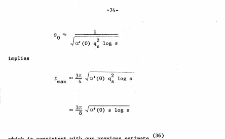
-4-relatively simple behavior of Regge trajectories in the direct channel.

The introduction of crossed-channel Regge trajectories can remove

difficulties arising from the high-energy behavior of high-spin

ex-changes. The relation of the direct-channel and crossed-channel

Regge trajectories, however, is not as simple as the relation, in the

static model, of direct-channel and crossed-channel fixed-spin

inter-mediate states. In fact, many Reggeized "models" fail even the simple

test of reducing to fixed-spin resonance models in the appropriate

kinematic region. Outside this region, one expects a crossed-channel

Reggeized model, for example, to be useful for describing processes at

high energies near the forward direction; the behavior at intermediate

energies and angles, however, is not easily treated in terms of Regge

trajectories: naive application of some of the standard formulations

of Regge pole theory can lead to impossibly difficult calculations.

If a scattering amplitude can be represented by an analytic

function, then the amplitude should be determined, in all channels, by

sufficiently precise specifications of its properties in only one

channel. For example, it should be possible to express the partial

wave amplitudes in one channel in terms of the set of partial wave

I amplitudes in another channel. The problem of the analytic

continu-ation of partial wave expansions is intimately connected with the

relation of Regge trajectories in two channels, since Regge poles arise

in a technique for the summation of these partial wave expansions.

In a practical implementation of any such continuation scheme, the

essential difficulties are associated with the fact that the physical

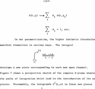
continuation of the partial wave expansion in any other channel, and the discontinuity across this cut is of fundamental physical interest. In other words, we are interested in determining the discontinuity of a function defined in terms of a (divergent) infinite series. In Section I of Part II, we introduce an analytic method which can be used to determine this discontinuity for a large class of Regge

representations, and in Sections II and III of Part II, we apply this method to some specific representations, for which we determine a

segment of the crossed-channel cut in terms of the distribution of Regge poles in the direct channel. Also discussed in Section I is a numerical method for the continuation of divergent partial wave sums.

In the phenomenology of strong interaction scattering, the observed sequence of bound states and resonances seems to indicate the indefinite rise of Regge trajectories with rising energy. By way of contrast, Regge trajectories in non-relativistic potential scatter-ing always turn around for high enough energy. In fact, some authors have supposed there to be difficulties in the phase shifts or analytic structure of scattering amplitudes, necessarily associated with

infinitely rising Regge trajectories. In Section I of Part II we show how the multi-sheeted analytic structure of the Regge trajectory function can be used to resolve these apparent paradoxes; added

-6-possibility which has been suggested by other arguments.

Section II of Part II is devoted to the application of the

mathematical apparatus developed in Section I to some Regge

repre-sentations introduced by other investigators. Specific strengths and

shortcomings of these fonnulations are examined. Two things are of

particular interest; first, the threshold behavior in direct and

crossed channels; second, the potentialities of these representations

for use in self-consistent or "bootstrap" calculations.

Finally, in Section III of Part II, a new representation is

introduced which surpasses the capabilities of the previous fonnulations

in these two areas. Just as in Section II, the mathematical devices

developed in Section I are applied to demonstrate their usefulness in

practical analysis. We show that the new representation automatically

satisfies direct-channel threshold constraints and can be made to

reproduce reasonable behavior of the discontinuity across the

crossed-channel cut. A scalar model is investigated for low energies, using

this new representation. In this discussion, we obtain a relation

between the mass of the lowest bound state and the slope of the Regge

PART I SECTION I

GENERAL REMARKS

Suppose that there exists a system of strongly interacting

particles obeying dynamical equations which have as solutions two

sets of masses and coupling constants. We are interested here in the

problem of spontaneous

su

3 syrmnetry breaking. In this case, one of

the conjectured solutions to the full dynamical equations would be an

su

3 syrmnetric arrangement of particle masses and coupling constants,

while the other solution would be the arrangement found in nature.

It is a moot point whether a complete and self-consistent

theory of elementary particles would have any solution except the

experimentally observed masses and coupling constants. Approximate

theories exist which have

su

3 syrmnetric solutions.( 2

) If we include

the features of an approximate model with an

su

3 syrmnetric solution,

the calculation will be internally consistent on this point. The

complete internal consistency of an incomplete theory is not necessarily

a reconnnendation, however, as we will see later in the discussion of

an overdetermined system of equations obtained in the theory of

spontaneous syrmnetry breaking.

Let A

1 and A2 be the scattering amplitudes corresponding to

the two solutions, where we have specialized to the partial wave, spin,

isospin, and strangeness appropriate to the bound states involved.

Using the N over D Method of Chew and Mandelstam, <3) we decompose

-8-A. (W)

l.

-1

Ni (W) Di (W) i

=

1, 2

We frame our theory using

w,

the center of mass energy, as the energy

variable. For each value of i, N. has the same

l. left hand cut (LHC) as

Ai but has no right hand cut (RHC), while D. similarly has a right

l.

hand cut but no left hand cut. The unitarity relation is

Im A. (U)

l. (RHC), i = 1, 2

from which follows

(RHC), i = 1, 2

( LHC), i = 1, 2

where p is a diagonal kinematic matrix, which is determined by the

definition of the amplitude in terms of the unitary S-matrix.

The D. will have simple zeros at the positions of the bound

l.

states and resonances. For simplicity, suppose that there is only

one bound state(4) and that the D functions are normalized to have unit derivative at the energy of the bound state:

(W-M.) 1

+

0 ((W-M.)2)

l. l.

for W ~ Mi' i = 1, 2

Now consider the function

J (W)

D~

(W) [A₂ (W) - A

At the bound states, the scattering amplitudes have poles

Ri

A. (W) "' ----~

+

smooth function

1 (W-Mi)

"' for W = M.

1 i = 1, 2

and, as a consequence,

and

Writing a dispersion relation for J(W) we obtain

J

ImJ(W)dW

+

.!. W-M. n

1

LHC RHC

J

ImJ(W)dW W-M.

1

i = 1, 2

where LHC and RHC designate the left-hand and right-hand cuts of J(W), respectively. Evidently, J(W) will have the cuts of both A

1(W) and A2(W).

Recalling that N(W) has no right-hand cut and that A = ND-l = DT-lNT (A is a synnnetric matrix due to time reversal invariance),' we can compute Im J(W) on the right-hand cut:

T Im J(W) = Im (D

2 (A2-A1) D1

J

T T

= Im (N

-10-On the left-hand cut,

where we have used the fact that D has no left-hand cut.

Finally, we obtain the equations

1

J

= -_:re LHC

DT

2 Im (A2-A1)

-=---,_...;'--'""""- D dW

+

!

(W-M.) 1 :re

l.

i

=

1, 2

Defining two new matrices as follows:

Evidently,

-1

l + ! (M2 - Ml)

n"

(Ml) +

Kl _{2 1}

and

-1

l + ! (Ml - M2) T" (M2) + • • •

K2

=

₂

Dz

Note that to solve the mass shift relations written above, 2

we would have to take weighted averages over 2N equations, where N

is the number of channels in the problem. There are obviously many

ways to construct these averages, and if there are errors present in 2

the original system of 2N equations, then there may be an optimum

weighting. Furthermore, the

~

elements of a residue matrix are not

all independent, but are completely determined by N coupling constants,

according to the factorization property:

Rij ₌ i gj _{i,,j 1, 2, N}

-gl 1 • 0 • '

Rij ₌ i gj -g2

2 2

In any calculation, the equations are approximated and the

overdeterminancy of the system requires serious consideration,

inde-pendent of assumptions about the size of the mass shifts and coupling

shifts. Again, what is indicated is a procedure for optimizing the process of selecting information from the overdetermined system with

errors.

As a step towarcs the solution of this problem, suppose

that some approximation to the residue shift equations were to yield

-12-su

3-breaking, R1 and M1 would be the residues and masses corresponding to the

su

3-synunetric limit, while R2 and M2 would represent the

corres-ponding quantities actually observed. In this case, R

1, M1, M2, and

any other necessary parameters might be specified initially or

deter-mined elsewhere in the general problem.

We can determine the factorizable matrix which is the

closest approximation to R

2, thus extracting from R2 a set of "coupling

constants." For simplicity, we choose the Euclidean metric as a

criterion of approximation. In other words, we want to determine a

set of numbers yi' i

=

1,2, ••• , N such that we minimize the expression

N

(Rij

€ _{= 2:}

i .. =l 2 l.J

Now observe that any matrix of the form

has two important properties. First, only one of the eigenvalues is

non-zero. Secondly, the vector y. is the eigenvector associated with l.

the non-zero eigenvalue. Evidently, a matrix which is intended to be

an approximation to a factorizable matrix would have to be

charac-terized by having one eigenvalue much larger than the rest. We will

assume this to be the case for

Ri

in the following discussion.

At a minimum, € considered as a function of the {y.} will l

possess a set of first partial derivatives all equal to zero.

i = 1, 2, ••• , N j=l

Decomposing R

2 into invariant sub-matrices, we obtain

where the numbers pK are the eigenvalues of R

2 and the vectors rK are the unit-normalized eigenvectors associated with those eigen-values.

Transforming to a basis where the matrix R

2 is diagonal, we see that the optimization equations may be written as follows:

N

(p. -

I

""'2 0 1, 2,

Yi l. yj) = i =

...

'

N

j=l

and

N N

E

=

L

[pi - 2PK -2 YK

+

-2 YK

I

-2] Yp,

K=l f,=l

where y is the transformed vector y.

It is now evident that the criteria for a minimum imply

±

;p;-

---J

max

i 1, 2, ••• , N

where by K we mean that value of K for which IPK attains max

max

the maximum value. The overall sign of the vector y. cannot be

-14-determined from the residue matrix.

In sunnnary, we have shown that a good approximation scheme to the residue shift equations must produce a real symmetric residue matrix which has one eigenvalue of much larger magnitude than the rest. Furthermore, the best way to obtain a set of coupling constants from this matrix, assuming our criterion for error, is to equate the coupling constants with the elements of the properly normalized eigenvector corresponding to the single largest eigenvalue. We also have obtained a measure of the deviation from factorizability in our approximate calculation

E

=

I

~K _max min

Factorizability is an important requirement for two reasons. First, i t expresses the fact that a single particle intermediate state

is present in the system, a dynamical condition that is central to our theory. Second, it communicates information among the N 2 elements of the residue matrix. Thus, if we have some way of extracting a preferred subset of equations out of the original N2 relations, we can partially compensate for lack of information about the remaining

elements by the imposition of factorizability using our eigenvector method. Specifically, we can search for a set of residue matrix elements which is consistent with our preferred set of residue shift relations and which, at the same time, most nearly satisfies factor-izability, minimizing ~

The mathematical development so far has placed no restric-tion on the size of the mass shifts or residue shifts. We have required only that the system possess two solutions and that the integrals involved be well-defined.<5) The accuracy of any calcu-lation using this mathematical framework is fundamentally limited by two things: first, by our knowledge of the amplitudes A. (and their

l.

decompositions N and D) on the left-hand and right-hand cuts; second, by the extent of the cuts we decide to include in the integrals for J(M.) together with the rapidity with which those integrals converge.

l.

In the actual calculation of coupling constants in spontaneous

su

3 symmetry breaking, we will use a model in which only single particle intermediate states are considered, whether in the direct or crossed channels. We will make many of the approximations characteristic of the so-called static model: static crossing relations, for example.

-16-PART I SECTION II THE MODEL

We will consider two body scattering of the baryon

su

3 octet

+

1(

-=

1/2 ) with the pion

su

3 octet PS (J

=

0 ) :

s-channel: _{BS+ PS} ~ B'

s

+ P'

s

t-channel: _BS+

B8

- P'

s

_{+ PS}

u-channel: _BS+

p~

~

B8 +PS

We will specialize to the £ = 1 partial wave. In this case, the total angular momentum can assume two values: Jn= 1/2+ and Jrc = 3/2+.

re

+

For J = 3/2 , there are ten states grouped in the baryon

su

3 decuplet,

. • 1(

+

The baryon octet itself has J = 1/2 •

We will assume isospin synnnetry and strangeness conservation

to hold in our calculation. Accordingly, it is not necessary to

differentiate different members of the same isospin multiplet. The

+

0

-isospin doublet (n,p) is referred to as N, the triplet (L ,

L , L )

is

called L, and so forth.

We will define a set of isospin coupling constants. The

coupling constant for a particular set of particles is obtained by

multiplying our isospin coupling constant by the appropriate

su

2

particle = g 0

pprc

isospin (~ 1 gNNrc ~ Z

1 1

2, z; 1, o}

The description of the B

8B8P8 and B8B10B8 vertices evidently requires twenty-nine coupling constants.

Five pairs of coupling constants, however, are constrained by charge

conjugation:

gNI:K =

• .f3/2

g.L:NK

1 1

gN/\.K

- J2

g11.Ni< gI:Arc =

"".[3

g/\.l:;TC

gz=:K =

- J°2/3

!FI:K

gA::::K =

J"2

~AK

We will not impose this constraint on the calculation; instead, we will

test whether i t is satisfied by our solutiono DDFS found that their

"enhanced eigenvector" of coupling constants was not markedly changed

when they projected out the parts violating charge conjugationo We

might expect to find a similar result. Of course, the charge

conju-gation information could easily be added to the list of preferred

equations, or i t could be a constraint imposed on the minimization of

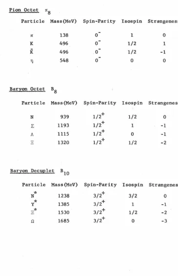
-18-Table 1 lists the particles in these three

su

3 families, each with its ma8s, spin, isospin, and strangeness. For the two baryon families, there is a tabulation of the channels in our

scattering system which can contain these particles as bound states or resonances. Our channels contain other resonances at higher energies, but we will limit our discussion to the two sets of states: B

8 and

It is characteristic of the low-energy limit of baryon-pion scattering that the i

=

1 s-channel crosses into the £

=

1 u-channel. This statement means that for £

=

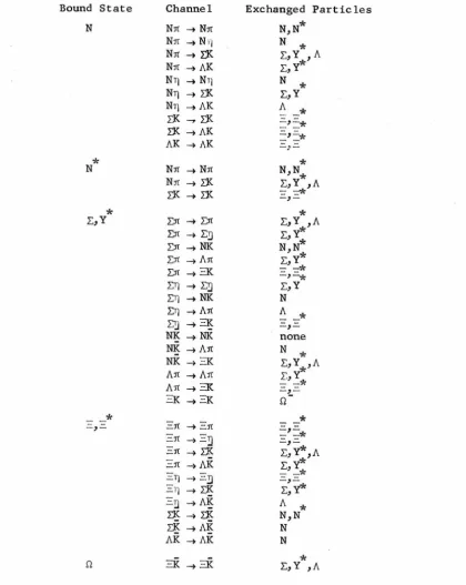
1 scattering the most influential u-channel states are precisely those particles bound in the s-channelo We assume that this low-energy behavior suitably represents the

behavior of the amplitudes at all energies involved in our calculationo We will neglect t-channel processes. Table 2 presents a list of all

the channels in our model, together with the resonances and bound states for each channel, and in every case the exchanged particles present as intermediate states in the u-channel.

We define our amplitudes by the following kinematic convention:

A=L

2i.q . 3

(S-1)

Since we are considering the case of broken

su

It was not considered worthwhile, ·however, to invest effort in improving

the detailed treatment of a model, such as the static model, whose basic

philosophy i's defective. Instead, in Part II, an alternative "simple"

model is developed which is more reasonable. The basic techniques of

Part I can be applied to any model. We use the static model mainly

because i t offers a simple illustration of these techniques and

secondarily, because it allows us to make a direct comparison with the

calculation of DDFS, which is also based on the static model.

A salient f~ature of our model is the assumption that, of

all the left-hand cuts, we need retain only the nearby short cuts

arising from baryon exchange. The left-hand cut contributions to the

J(M.) are then written as functions of the masses and residues of the

]_

exchanged particles. Since the system of particles that is exchanged

is the same as the system that appears as bound states, the mass-shift

and residue-shift equations form a closed algebraic system which can be

solved to determine the masses and residues of the natural set of

baryons in terms of a fictitious

su

3 symmetric baryon system. If the

equations derived from this approximate model were completely

self-consistent, then the overdeterminancy of the system would be no problem.

In general, however, we expect errors to be present which render our

approximate equations inconsistent.

If the mass shifts and residue shifts are assumed to be

sufficiently small, then we could use a perturbative approach, such as

that investigated by DDFS. The experimental baryon octet and decuplet

masses vary less than about fifteen percent from their average values.

-20-in the mass shifts. Correspond-20-ing experimental measurements of couplings are less precise, but the calculations performed in DDFS(6) yielded coupling shifts as large as the

su

3 synunetric couplings. This situation would seem to rule out perturbative or power series ap-proaches for the coupling shifts.

In their linearized theory, DDFS noted that the integrals in their coupling shift equations would converge faster than those in their-mass-shift equations, by a power of W. This feature may carry over into our theory. The residue shift equations could be more ac-curate than the mass shift equations, since they are one higher order in the perturbation. This possibility would be realized only if all orders in the coupling shifts were kept for each order in the mass shift expansion. Within the limits of our approximate model this is the case. If synunetry breaking is relatively larger at low energies than at high energies, this effect would be enhanced. Accordingly, we will perform only the residue shift calculation, since our model does not adequately treat distant cuts. Whenever they are needed, the mass shifts will be taken from experimental data. After we have

obtained the residue shifts, we will determine the errors in the mass shift equations when we make the same approximations used in the

coupling shift calculation. This procedure will provide a rough check on the self-consistency of the approximations involved in our calcu-lation.

of the right-hand cut appears in first and higher orders, but not in zeroth order. Several authors have remarked that the calculation of the contribution of the right-hand cut is extremely model-dependent.(]) DDFS, in their treatment of residue shifts, avoided explicit treat-ment of the right-hand cut.

series:

Near the bound state we can expand the D.(W) in a power ].

D. (W) _]. = (W-M.) 1

+ -

₂1 (W-M. )2 D." (M.)

+ .•.•

]. ]. ]. ].

The nearest singularity of D.(W) is at threshold. In an exact

calcu-1

lation, the second and higher order derivatives of

n

2(W) would include effects of the residue shifts, as well as mass-shift effects.

Following DDFS, we choose to ignore the cut in Di(W) for purposes of computations on the left-hand cuts of Ai. We retain only the nearby short left-hand cut resulting from bayon octet and decuplet exchanges. If the scattering process involves a baryon of mass M

a and meson of mass µa scattering to form a baryon of mass ~ and meson of mass µb' an exchange of a baryon of mass Mexch will produce a short cut running from £ _exc h =

.fs

_- to µ _exc h =

.fs+

where (8)

-cr

4

+

t

(cl+13+/+0

2

) + CX13y6

±.J

(cr2-o:

2

)(cr2-13

2

)(cr2-/)(cr2-o

2)

2cr2

0:

y

-22-For Won this leit-hand cut, !W-Mil is of the same order of magnitude

as the observed mass shifts.

In the following calculation, we will keep only the lowest

terms in (M

1-M2). Accordingly, we drop the second and higher order

terms in the expansion of D.(W) on the short left-hand cut, thus

obtain-1

ing the so-called "linear-D" approximation. Within any specific model,

of course, D.(W) can be calculated and included accurately, necessitating

l.

a nonessential modification of the following discussion. Evidently,

we can set K

1

=

K2

=

1 consistent with keeping (M1-M2) only to lowest

order. This assumption also allows us to neglect the right hand cut.

In the above approximations, the residue shift equations

become:

oR

I;

ex ch

where by X we mean all terms not specifically included.

The mass shift equations become:

~

_rclfµexch

~ dW (W-Mz)(Im A2 - Im Al)

ex ch

fl,exch

+

x

~

_rel

Jµ

ex ch

~ dW (W-M

1)(Im A2 - Im A1)

ex ch

fl,exch

+x

In the static model, the short left-hand cut is approximated

~t

I I u

J

m A~W~dW 1 1 ' I

e! _{Im A (W) dW}

(W-w)

<

w

> -

w

:n:

p, _p,

1

R

<

W >-W exch

or

1 I "'

n

Im A

2 (W) R

ex ch (u-£)

where R h is the residue of the amplitude in the u-channel.

exc

So we can write:

oR = OR _exc h

+

X

Using the static crossing relations, which relate states of angular momentum £ = 1 in the s-channel to states of £ = 1 in the u-channel, we can determine R h from the residue of the bound state

exc in the crossed channel.

oR = CoR

ex ch

where C depends on the spin and isospin of the direct and crossed channels.

In writing this equation, we have assumed the crossing

matrix is the same for the

su

3 symmetric and unsyrnmetric cases. This asslllllption is equivalent to neglecting higher orders in

(M

2-M1) in the crossing matrix.

Finally, our equations become

-24-Except for terms in the vector

x,

these equations along with the factorization constraint are unchanged if all residues R

2 and R1 are multiplied by the same factor; they are likewise independent of the

particle masses.

As an illustration, consider the process L)r .... NK for

£ = 1. In the direct reaction are channels having isospins I=

o,

1 and spins J = 1/2, 3/2. Of the particles in the baryon octet and decuplet,

6,

A, Y*

are found as intermediate states. The crossed reaction with nonzero baryon number is ~K-.

Nn.

Possible isospin and spin states with£= 1 are I = 1/2, 3/2 and J = 1/2, 3/2. N and N* are found in the crossed channel. Consequently, we say that the scattering amplitudes for ~rt -. NK have two short left-hand cuts which arise from the exchange of N and N*. To calculate the crossing matrix, consider a particular charge state of the process in the s-channel:

~+

n

°

..

pK 0

This channel is purely I 1. Consulting a table of Clebsch-Gordon coefficients, we obtain

no

I

A

I

pKo)

=.rt

Crossing, we obtain the u-channel process:

This reaction is evidently a mixture of I = 1/2 and I 3/2. From a table we obtain

.[2

u

.[2

u

Consequently we can write

2 u 2 u

=

3

AI=3/2 -

3

AI=l/2

Similar calculations applied to the process ~0n° ~ nK

0 allow us to obtain the behavior of A~=O under crossing. States of orbital

angular momentum £ = 1 cross into themselves in the static limit, so we want to calculate the crossing of s-channel states with J = 1/2, 3/2

into u-channel states with J = 1/2, 3/2. Spin crosses the same way as isospin in the static limit, and a claculation similar to the isospin calculation above yields

s 2 u 1 u

AJ=3/2 =

3

AJ=l/2

+

3

AJ=3/2

2 1 u 4 u

AJ=l/2 =

-3

AJ=l/2

+

3

AJ=3/2

Combining the crossing relations for spin with those for isospin, we obtain crossing relations for the particle states in the direct and crossed channels:

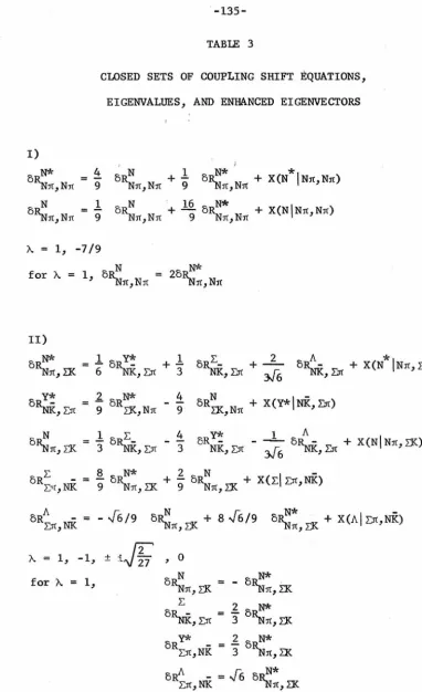
= 8

.f6

9 Au -~.,., _.f6Au 9 -~

-26-5R(Y*IL.:rr, NK)

=

9

2 5R(N* IN1r, L.K)

- 9

4 5R(NIN:rr, L.K)

+

X(Y* /Dr, NI<)

5R(L. Jr.:rr, NI<)

~

5R(N* IN1t, l.:K)

+

g

2 5R(NJN1r, L.:K)

+

x

(Y~" I r.n, NR)

5R(A J2::1r, NI<)

=

8

~

6 5R(N*INn,r.K) -

.[~

5R(N INlr, L.K)

+

X (A 1r.n, NI<)

A complete list of our residue shift equations for baryon-pion scattering is given in Table 3. Note that there are 74 equations but, assmning factorization, 29 independent unknowns (assuming charge conjugation invariance, this number drops to 24).

DDFS did not explicitly consider the problems associated with the inconsistency of the residue shift equations. They made the approximation

thus linearizing the residue shift equations in 5g (discarding terms 1

which were not negligible), and then projected the gi out against itself (an averaging process -which is not necessarily optimal). The resulting equations were treated by matrix methods. In this approx i-mation the matrix R

2 is automatically factorizable. The equations for the coupling shifts were written in the form

og. = A~~ 5g .

+

X.

1 1J J 1

the treatment of the equations; and possibly, from interactions present in nature which break

su

3 in the same way that the presence of electromagnetic interactions break isospin symmetry. Not expecting to be able to calculate X accurately, DDFS noted that if Agg has an eigenvalue near one, the projection of the corresponding eigenvector on the vector X will be much larger than projections of X on the other eigenvectors, except for the case, of low probability, where the un-known vector X happens to be orthogonal to the favored eigenvector. The eigenvector corresponding to the unit eigenvalue of Agg is said by DDFS to be "enhanced." The elements of this eigenvector will probably be nearly in the same ratio as the coupling shifts observed in nature. The overall magnitude of the coupling shifts, however, can be determined only from unattainable knowledge about X. This procedure is suspect for finite coupling shifts if X is itself a rapidly varying function of the coupling shifts.

DDFS, in selecting an enhanced eigenvector of Agg' arrived at a process of filtering information out of the over-determined system with errors. Their method, however, derives from an invalid linearization of the original equations as well as an averaging of these equations which is not necessarily optimal. We expect it to be accurate, at best, in the limit of small coupling shifts; i t may give only a rough estimate of the full-size coupling shifts.

Our method, on the other hand, is not limited to linear systems. The factorizability of R

PART I SECTION III THE CALCULATION

In the following pages, we apply the principles developed in Section I to the model discussed in Section II. In Table 3, the residue shift equations are arranged in closed systems of linear equations, the coefficients being determined from the crossing matrix elements. As before, the equations are written in the form

5R A5R

+

X

so that the homogeneous equations have a solution when the matrix A has an eigenvalue equal to one. Table 3 lists the eigenvalues of the matrices A, and in those cases where an eigenvalue is near one, the

eigenvector corresponding to that eigenvalue is also tabulated. Note that in almost every case, (9) there is a clear

differentiation between systems with an eigenvalue near one and systems with no eigenvalue near one. The single exception is a system with

an eigenvalue ~ ~ .69, which was assumed to be close enough to one to warrant including the corresponding eigenvector in the set of pre-ferred equations.

Proceeding by the same logic as DDFS, we assign a special significance to the eigenvectors corresponding to the eigenvalues near one; we expect that the residue shifts are roughly proportional to the elements of these eigenvectors, subject to the constraint that the final residue matrix, R

-30-Table 4 contains a list of equations obtained by assuming that the residue shifts are proportional to the enhanced eigenvectors. Note that in going from the equations in Table 3 to the set in Table 4, we have reduced the number of equations from 74 to 38. Assuming that

the equations in Table 3 explicitly include all the important terms varying with DR, we expect a reduction of errors concomitant with the reduction in the number of equations.

Following DDFS, we refer to the selection of the smaller number of equations as nenhancement." Not every residue shift is

enhanced; some residue shifts are not determined by the equations in Table 4. We shall require that the unenhanced elements of the residue matrix R

2 be chosen to minimize the deviation of R2 from factorizability. In this respect, we will be concerned with a second set of eigenvectors: the eigenvectors of the matrix R

2•

The equations in Table 4 can be arranged so that the enhanced elements of the baryon octet residue shifts are determined by the

decuplet residue shifts. There are twelve decuplet-baryon-pion coupling constants. Writing the decuplet residues in terms of the decuplet

coupling constants, we insure that the decuplet residue matrices are factorizable; the octet residues are determined by these twelve para-meters, but are not necessarily factorizable.

decuplet coupling constant as well. Fixing this number at an experi-mental value corresponds to specifying the size of the perturbation

in the calculation of DDFS.

In sunmtary, the original problem involving 74 equations in 29 unknowns has been reduced to a minimization problem in eleven variables. The actual calculation proceeded by an iteration scheme. The results of the DDFS calculation were used as a starting point for the matrix R

2• The unperturbed residue matrix R1 was fixed according to the

su3

syrmnetric model.

The enhanced octet matrix elements were replaced by the values indicated by the equations in Table 4, the present values of the decuplet residue elements being taken as input.

The

Ri

resulting from this modification was then diagonalized and an optimum factorized approximation was computed, according to the methods discussed in Part I. We designate by Q this factorized approxi-mation to R

2• Briefly,

and

K K

=L:pKA.A.

K i. J

where I: i

If the choice of the eleven decuplet couplings were perfect, and the original equations were completely self-consistent, then Q and R

2 would be identical. The discussion in Part I indicated that a reasonable measure of the deviation of Q from R

-32-€ ₌

In our actual calculation, we used another measure of the deviation:

€ _{= L:}

IQ .. -

_(R2);J·

I

. . iJ .L iJ

min

This step was taken because i t was felt that the quadratic measure was

insensitive to the behavior of couplings whose absolute magnitudes

are much smaller than the average. Even with a linear measure, some

insensitivity was evidenced (see Table 5).

The eleven-dimensional gradient of the error criterion,

€ . , was then computed by varying slightly the eleven free decuplet min

coupling constants and computing the values of R

2,

Q,

and €min at each

point.

The unenhanced matrix elements of R

2 were then replaced by

the corresponding elements of

Q,

and the decuplet couplings were moved

a reasonable mesh step along the gradient of € . • min

The iteration consisted of returning to the calculation of

the enhanced matrix elements of R

2 from the equations in Table 4. This

process was continued until the norm of the gradient of the error

criterion fell below a satisfactory level, indicating that R

2 had been

optimized with respect to factorizability. One cycle of this iteration

process required from six to ten seconds of 7094 computation time.

Sixty iterations were performed in the calculation.

Notice that the computation centers around the diagonalization

matrices, before and after application of the optimum factorization

procedure. Also listed are the eigenvalues of each residue matrix.

Ideally, only one eigenvalue would be non-zero. Our optimization

procedure makes one eigenvalue much larger than the rest.

Table 6 contains a list of the

su

3 symmetric couplings,

the couplings obtained in DDFS, and the couplings obtained in this

calculation. In most cases, this calculation agrees with DDFS on

the direction of coupling shifts away from the

su3

symmetric limit;

we obtain, however, different magnitudes of shiftsa This result is

consistent with our expectations.

As a check of the charge conjugation properties of our

couplings, Table 7 compares the theoretical ratios with the results of

our calculation. The charge conjugation ratios could have been taken as

additional constraints on our set of eleven free decuplet couplingso

Otherwise, we could follow the example of DDFS and average out the

charge conjugation errors.

As an additional check on the residue calculation, we

investigated the consistency of the mass shift equations. Table 8

lists the masses computed from the experimental masses and the

calcu-lated coupling constants. To test the sensitivity of our calculation

to the neglect of kinematic effects in the crossing matrix, we performed

the same computation using the static model crossing matrices including

the correct kinematic factors determined by experimental masses. As

can be seen in Table 8, the masses were not very sensitive-to these

PART II SECTION I GENERAL DISCUSSION

Consider the two body elastic scattering of spinless particles

of identical nonzero mass, M. There are three physical channels:

s-channel: 1 + 2 _. 3 + 4

t-channel: 1+3~2+4

u-channel:

We will find it convenient to use the standard Mandelstam variables:

s, t, and u, the squares of the total CM energies in the s-channel,

t-channel, and u-channel, respectively. We will also use the squares

of the CM momenta: Finally, we will use the cosines of

the CM scattering angles in the various channels: cos

es,

cos et,

cos

e •

u

following:

These variables are related by equations such as the

s = 4(q2 + M_s 2) 2

e )

t = -2q (1 - cos

s s

2

e )

u -2q (1

+

cos

s s

The Mandelstam variables are constrained as follows:

2 s + t + u - 4 M

-36-amplitude is a function of only two independent variables.

We assume that the scattering amplitudes are analytic

func-tions of the Mandelstam variables, except for cuts and poles, and that

the scattering amplitude for any channel can be obtained by analytic

continuation of the amplitude for any other channel, so that one

amplitude is sufficient to determine the scattering in all three

channels. We do not admit the possibility of natural boundaries in our

scattering amplitude~

In any channel, the scattering amplitude can be expanded in

a Legendre series. For example, in the s-channel

00

A (s, t,u) = E (2£

+

1) a (s) P£ (cos

e

)

£=0 £ s

s

>

4 M2

- 1

<

cos

e

<

1 s

The sum converges for all physical s-channel angles, provided that all

crossed-channel intermediate states have nonzero mass. This

require-ment means that our idealized scattering process does not include

electromagnetic interactions, for example.

It is convenient to work with kinematic singularity free

amplitudes. In this case, the scattering amplitude will have a

singu-larity if and only if one of the Mandelstam variables attains such a

value that a physical intermediate state is possible. For example, if

there is a single particle state of mass M , whose quantum numbers are x

2

s

=

~· A trivial set of multiparticle states are the two-body

intermediate states consisting of particles 1 and 2 in the a-channel. These states cause the scattering amplitude to have a cut running from

2

s

=

4M to s

=

oo • In general, an a-channel multibody intermediate

state of N particles with masses Mi' i cut in the amplitude running from s = take all such cuts along the real axis.

2, ••• ' M. )2 to

1

N will produce a s = oo • We will

Of particular interest is the case where the scattering is defined in terms of a set of partial wave amplitudes. For physical a-channel angles, the set completely specifies the total amplitude according to the convergent Legendre series. This set is thus suf-ficient to determine the scattering amplitude everywhere, by means of analytic continuation. The various techniques of this analytic

continuation are a central topic of our later discussion.

At this point, i t is appropriate to review briefly the Sommerfeld-Watson transformation, a classic technique for the continu-ation of the Legendre series.(lO) An analytic function can be found which interpolates the partial wave set( a£(s)} in a strip containing

the positive real £-axis. We designate this function by a£(s), and henceforth our notation will not differentiate between the set of partial wave amplitudes and any interpolation we might choose. Then the Legendre series can be written as a contour integral:

00

L

(U+l) a£ (s) P£ (s) £ = 0

<)._(s) P~(-cos es) (2~ + 1) sinrr~

-38-counterclockwise around the origin and back to oo above the real axis.

c

is chosen to lie entirely inside the strip of analyticity of a£(s). It should be evident that interpolation is not unique. We will require, however, that a£(s) be chosen in such a way that

J

c'

dA (2A+l) a,._(s) PA (-cos es)

Sin n A = 0

where C' is the arc of infinite radius centered on A = -1/2, extending clockwise from A

=

-1/2 + i oo to A

=

-1/2 -i oo • It has been

demon-strated ( ll) in the theory of potential scattering that there is at most one function a£(s) which satisfies all these requirements, and that such a function will be analytic in the £-plane except for poles. Then we can express our Legendre series in terms of a finite series

and another contour integral: 00

I

£=0

2a +l n

sin

n

a

~n Pan (-cos es) n

dA a,._(s) PA(-cos es) 2i sin n A C"

C" is a straight line running from A

=

-1/2 + i oo to A

=

-1/2 -i oo •

These trajectories have a special physical significance.

As we vary s, the set of Regge poles will move along their trajectories. Fixing £ at some non-negative integer, we see that the partial wave amplitude a£(s) appears to go through a resonance as any of the trajectories passes near£. Evidently, there is pole dominance near a resonance. As we shall see later, however, i t would be incorrect to assume that any pole or finite collection of poles in this expansion accurately represents non-resonant amplitudes.

Of particular consequence is the importance of the Regge pole terms relative to the contribution of the background integral. It can be shown that the Regge pole terms dominate the background integral as jcos Bsl ~ oo • In fact, the asymptotic behavior in

cos

e

is determined by the asymptotic expansion of the leading pole

s

terms, for which Re

a

is maximum: n

A(s,t,u) I

2n 13 n

cos es , _.. 00 sin ncx n

r(a

+3/2) n

r(

a

+

1) n

0:

(2 cos

e

)

n s

For finite cos es, however, the other trajectories and the background integral are important. If we are concerned with low-energy behavior in the t-channel, the Sonnnerfeld-Watson transformation is especially clumsy.

Suppose that Mx is the mass of the lowest-energy

inter-mediate state in the crossed channels (not necessarily a single particle state). Without any essential loss of generality, we can consider the

' (12)

-40-wave expansion will converge inside an ellipse in the complex cos

e

-s

plane with focii at cos

es

= ± 1 and whose boundary includes the M2

nearest singularity, cos

e

_s = 1

+

~-x

2

• This point corresponds to an 2q

unphysical angle. s

It is convenient to define a function s(s):

cosh s (s)

s

(s)

>

0

The function represented by our Legendre series then has a singularity

at cos

e

= cosh s(s). For simplicity, suppose that this singularity s

is a pole. Later on, we can integrate over a distribution of poles to

represent a cut.

The contribution of the pole to the partial wave amplitude

is

where p(s) is the residue of the pole int:

(

) -E..hl+

A s,t,u

2 t-M

x

for t M2

x

regular function

The nearest singularity dominates the asymptotic behavior

of the partial wave amplitudes as£ ~oo, Re£> - 1/2 •

asymptotic behavior of Q£ we obtain(l3)

From the

. . . 00

Re £

>

-1/2

exp

r-

(.?+1/2)

s

(s)]

.. .ju

sinh

~

(s)

The more distant singularities contribute terms whose magnitudes decrease at exponentially faster rates as

.e

~ oo •

Approximating the Sommerfeld-Watson expansion with a single Regge pole results in the following partial wave amplitudes:

p

(2a +l) n n

(a -.e) (a H+l)

n n

Evidently this approximate amplitude has incorrect asymptotic behavior

as

.e __.

oo _{This property corresponds to an improper positioning of}

singularities in the cos es-plane. Pa(-cos es) has a cut running from cos

e

= 1 to cos

e

= 00

s s This extraneous cut from cos

e

s = 1 to cos

e

cosh ~(s) can be removed by adjustment of terms between the

s

Regge poles· and the background integral. (l4) In this case, the pro-blems remain of imposing direct-channel unitarity and determining the background integral in terms of physically relevant quantities. The behavior of the amplitude near cos

e

= cosh ~(s) is not well

approxi-s

mated by the Sommerfeld-Watson representation, and for physical s-channel angles we would expect the method to be even worse.

We adopt the customary definitions of phase shift 5.e and elasticity TJ.e in terms of the S-matrix projection S_e, as follows:

1

-42-Log Sp, is purely imaginary above threshold for a process with no open inelastic channels.

In every case,

p, =

o,

1, 2, •••

Definition of the amplitude in terms of a unitary scattering matrix is a matter of convention. With some choice of kinematic factor,

K(s), we can write

1

= 2 iK ( s) [ Sp, ( s) -1] •

From the asymptotic behavior of the scattering amplitude, we obtain

log Sp,

f, .... 00

i p(s~ K(s)

J"rr.

exp [-(J,+ 1/2) s(s)] qs

JU

sinh s (s)

Re p,> -1/2

We could generalize this asymptotic formula by writing an expansion of log Sp,, which explicitly exhibits the relationship between the detailed behavior as P, ... w and the singularity structure of the

amplitude in the cos

e

-plane: s

log Sp,

=

I:

n

er

<s )

z

<

£

, s )

n n

+

J

00

d<'

a(~')

z (£

,<')

s

where the sum is taken over the s (s) corresponding to single particle n

cos

e

plane. Evidently for the nearest singularities s

p, ... 00

Re P,

>

-1/2

but the precise form of Z(P,,s) would have to be determined by a more careful study of the asymptotic properties of log Sp, • If the

scattering in a certain energy region of the crossed-channel process were dominated by a resonance, i t would be valid to write a resonance

approximation to the integral:

JdS' a(S ') Z(£,S) ;:' R(£R) Z(£,£R) •

s

For a wide class of potential scattering problems, i t has been demonstrated(lS) that the asymptotic behavior of Sp, in the left-half P, -plane is

Sp, ~ exp [2i rt(P,+ 1/2)]

Re P,

<

-1/2

-.

44-£-plane, however, indicates that the background integral would thereby become more important, rather than diminish.(l7) Such a process would therefore not be convergent. We are forced to the conclusion that the background integral is important and is not simply related to the Regge poles that lie to the left of the.background integral contour.

tude is

The elastic unitarity condition for the partial wave

ampli-2

= K(s) lat(s)i £ =

o,

1, 2, • . • •

This equation is a hopeless tangle of Regge poles and background terms, unless we restrict our consideration to a small number of terms in the Sommerfeld-Watson expansion. In channels with no inelasticity, the unitarity condition can be written for complex £

s*

(s)

s

(s)

=

1 £* p,

2

s, ~ 4 M

Therefore elastic unitarity implies that if Sp,(s) has a pole at

*

p, = a(s), then it must have a zero at P, =

a

(s), and under no other circumstances. The Regge pole structure of the S-matrix determines in a trivial way the positions of all the poles and zeros of the S-matrix. The corresponding statement is not true for the amplitude, however.

The most natural way to incorporate this information into the amplitude is to use a product form(lS) for St :

.e

-

a

(s)

(

*

)

~

.e-

a

: (s)

<I> n (s)

x-,n

where the product is taken over the Regge poles of the amplitude. The <l>n are convergence factors. We could write this relation as

x-,n

follows:

log S,e =

where

*

=log

[(£-a

(s)] -log

[£-a

(s)]

n n

+

<Ii n (s) x-,n

From our previous discussion, we impose asymptotic conditions on

I: n

\fr £,n £

ip(s) K(s).frt exp[-(£+ 1/2)5] q;

.J

22 sinh

~

I: \If n x-,n

n

.... 00

Re £

>

-1/2

£ ... 00

Re £

<

-1/2

2i rt(£ + 1/2)

Elastic unitarity is equivalent to

Re = 0

n

In the general case, we must have

Re I: 1jr £ n

:S.

0

'

o,

1, 2, . • . .

-46-The only finite singularities allowed for

t

,,,

n

,n

are logarithmic singularities at the Regge pole and Regge zero. The requirement that the Regge singularity in the amplitude be a simple pole fixes the overall multiplicative constant for

W

,,,

n

,n

•

This fact will have a bearing on the size of p(s), the t-channel residue of the whole amplitude. ~n is not defined as an analytic function of s

,,,

,n

*

'

*

unless we replace

ex

~ an analytic function agreeing with

ex

(s) for

n n

real s above threshold. Such a function is ex11(s), the anlytic con-n

tinuation of

ex

(s) defined by taking a counterclockwise circuit around n

the threshold branch point and onto the second physical sheet. To avoid any confusion, we denote the function

ex

(s) on the first physical

n

sheet by ex1(s). We should then express

Wn

(s) in terms of the boundary

n .,n

values of the analytic functions

Wf,

n(s) = lirn {log [£-ex11(cr)) - log [£-ex1(cr))

, € -+ 0

This point is important, as we will see later in a discussion of the effects of open inelastic channels.

Just as in Part I, our concern here should be to make maximwn use of the information we possess about our scattering

pro-cess, and to cast the approximation scheme in such a way as to minimize the consequences of errors we will inevitably make in

In order to satisfy unitarity, we have introduced a "Regge

zero" as well as a Regge pole, and thereby have lost the possibility

of independently specifying a Regge residue. Near a Regge pole, in

fact:

s

(£' s) = e

I

cfln(cxn,s)( I

II)

ex -ex

n n I p,

-ex

n

n

m=#n

for

.e

= cxI n

+

regular function

As we remarked earlier, all that is necessary for a complete

specification of the total scattering amplitude is knowledge of the set

of partial wave amplitudes (ap,(s)} for non-negative

.e,

along with a

viable method of analytic continuation. We have rejected the

Sommerfeld-Watson transformation for practical reasons: it is clumsy in dealing

with direct-channel unitarity and in determining the behavior of the

amplitude around nearby crossed-channel singularities, and there is

no simple way to approximate the background integral. Another reason

for searching for different techniques is that the Sommerfeld-Watson

method involves the use of unphysical scattering amplitudes. It is

fashionable in S-matrix theory to take care to talk only about

physically relevant quantities; at the critical step, the relation

of one channel to another, it seems odd to reso'rt to unphysical

entities, such as the values of

a.e

·

for Re£= -1/2.

We shall, however, utilize certain information abstracted

-48-consideration to a class of representations for the scattering

ampli-tudes for which Regge poles are manifest, thereby treating whole

sequences of resonances in a unified way. We also incorporate

non-Regge information, insisting on certain asymptotic behavior of our

amplitudes, independent of the level of approximation.

We will make use of representations in which log Si is

specified in terms of physically relevant quantities. In this case,

log Si is a simpler function than Si' from the point of view of

practical analytic methods. Nevertheless, we must continue the sum:

A(S, cos

e )

= s

00

l

~

(2i

+

1) {exp [log Si(s)]-l}P (cos es) 2i K(s) i=l

Let us therefore consider a class of methods for the continuation of

functions defined in terms of Legendre series. It will be obvious that

these methods, with appropriate modification, can be used for expansions

in terms of any set of orthogonal functions.

Consider the analytic continuation of

f(z)

where the related function

g(z) ~ (2£

+

1) b£ P (z) i=O

will yield more readily to analysis. Writing Cauchy formulas for

1 f(z) = _re

1

g(f)

=

_re

r

z 0

dz' 6f(z') z'-z

dz' Ag(z') z'-z

we want to determine 6f(z) in terms of 6g(z). We define a new

function;

which for 0

<

A ~ 1 evidently converges within the same region as the

sum for f(z). Trivially, f

0(z) = 0 and f1(z) = f(z). Differentiating the new function, we obtain

= g(z)

+

Now we have obtained a new Legendre series whose coefficients are

products of coefficients belonging to two other series.

Recall the addition theorem(l9) for Legendre polynomials:

p,

p (z") _{p, =} p ( ) p ( •) _{p, z p, z}

+

2 L: _(P,+m) (f,-m)

~

_~ pm ( ) Pm( ') _{p, z p, z cos m} <!> m=l

where z"

Also recall the •orthogonality condition(20) for the Legendre

1

r

p£ (z) p£ I (z) dz =

c./ -1

-so-2 f>.e,e•

u

+

1

These two properties imply that our new series can be

expressed as follows:

00 ~b.e

~

(2£

+

1) b.e(e

-1) P.e(z)

£=0

= _4n 1

J

-1 1

dz'

J

0

d<)) f (z' )g(z") ~

1 2 .!. 2

a

z"=zz '+(z -l)z (z' -l)cos <))

Consequently, we have reduced the pr