Energetic Variational Approaches
J Brannick, A Kirshtein, and C Liu,Penn State University, University Park, PA, USA
r2016 Elsevier Inc. All rights reserved.
Introduction 1
1 Two Fluids Mixture 2
2 Boundary Conditions 4
3 Mixture of Three Fluids 5
References 6
Introduction
Complex fluids are those with internal microstructures whose evolution affects the macroscopic dynamics of the material, especially the rheology. Examples include polymer solutions and melts, liquid crystals, gels, suspensions, emulsions and micellar solutions (Larson, 1999). Such materials often have great practical utility since the microstructure can be manipulated via processing of theflow in order to produce useful mechanical, optical or thermal properties. An important way of utilizing complex fluids is through composites. By blending two immiscible components together, one may derive novel or enhanced properties from the composite, and this is often a more economical route to new materials than synthesis. Moreover, the properties of composites may be tuned to suit a particular application by varying the composition, concentration and, most importantly, the phase morphology. Perhaps the most important of such composites are polymer blends (Utracki and Favis, 1989). Under optimal processing conditions, the dispersed phase is stretched into afibrillar morphology. Upon solidification, the longfibers act as in situ reinforcement and impart great strength to the composite. The effect is particularly strong if thefibrillar phase is a liquid-crystalline polymer (National Materials Advisory Board,National Research Council, 1990). Another example is polymer-dispersed liquid crystals, with liquid crystal droplets embedded in a polymer matrix, which have shown great potential in electro-optical appli-cations (West, 1990).
From a fundamental viewpoint, such composites are extremely interesting. They feature dynamic coupling of three disparate length scales: molecular or supramolecular conformation inside each component, mesoscopic interfacial morphology and mac-roscopic hydrodynamics. The complexity of such materials has for the most part prohibited theoretical and numerical analysis. The main difficulty is the moving and deforming interface between the two components. Traditionalfluid dynamics treats these as sharp interfaces on which matching conditions must be imposed.
There are various approaches that have been developed to model complexflows. The boundary integral and boundary element methods use a mesh with grid points that lie on the interfaces and deforms according to theflow on both sides of the boundary (Cristini et al., 1998;Toose et al., 1995;Kelly et al., 1983). These include works onfinite-element methods (Hu et al., 2001; Ambravaneswaranet al., 2002;Hooperet al., 2001a,b; Kim and Han, 2001) andfinite-difference methods (Ramaswamy and Leal, 1999b,a). Two drawbacks of these approaches are that keeping track of the moving mesh can entail a large computational overhead and large displacement of internal domains can result in mesh entanglement as happens, say, when one drop overtakes another. Typically, a remeshing scheme is activated, introducing geometric error into the discrete approximation (interpolation error) as well as additional computational cost. Most importantly, the moving-mesh methods cannot handle singular morpho-logical changes such as breakup, coalescence, and reconnection; the sharp interface formulation breaks down in such cases. Thus, these methods have so far been limited mostly to single drops undergoing relatively mild deformations.
As an alternative,fixed-grid methods that regularize the interface have been highly successful in treating deforming interfaces. These include the volume-of-fluid (VOF) method (Li and Renardy, 2000a), the front-tracking method (Unverdi and Tryggvason, 1992) and the level-set method (Sethian and Smereka, 2003;Zheng and Zhang, 2000;Changet al., 1996). Instead of formulating theflow of two domains separated by an interface, these methods represent the interfacial tension as a body force or bulk stress spread over a narrow region covering the interface. Then a single set of governing equations can be written over the entire domain which can be solved on afixed grid in a purely Eulerian framework, as inLi and Renardy (2000b); the overview paper (Sethian and Smereka, 2003) gives an insightful comparison of such approaches.
☆Change History: June 2015. C. Liu, J. Brannick and A. Kirshtein made minor typo, formatting and other pre-submission corrections. Changed links tofigures
1–2 in the text, and changed the energy dissipation and boundary conditions in section 2 (Boundary conditions) to a more conventional form.
Here we focus on the diffusive interface method, which uses a phasefield to smoothen the transition between two phases (Liu and Shen, 2003). The approach can be viewed as a physically motivated level-set method. Instead of choosing an artificial smoothing function for the interface, which affects the results in non-trivial ways if the radius of interfacial curvature approaches that of the interfacial thickness (Lowengrub and Truskinovsky, 1998), the diffuse interface model describes the interface by a mixing energy. This idea can be traced tovan der Waals (1979), (first published in 1892), it has been widely used and successfully incorporated to numerous practical applications, including models of phase transitions (Hohenberg and Halperin, 1977; Cagi-nalp, 1986;Wheeleret al., 1992), contact line dynamics in complexfluids (Liu and Shen, 2003;Qianet al., 2003,2006;Brannick et al., 2015;Yueet al., 2004), cell motility (Aronson, 2014), and many other problems in science and engineering. Thus, the structure of the interface is determined by molecular forces; in particular, the tendencies for mixing and demixing are balanced through the non-local mixing energy. Moreover, when the capillary width approaches zero, the diffuse interface model becomes identical to a sharp interface level-set formulation. The method also reduces properly to the classical sharp interface model.
To build a diffusive interface model of complexfluidflow, one can use concentration, mass fraction or volume fraction as a phasefield and builds a model based on conservation of mass, conservation of momentum and other physical assumptions (Lowengrub and Truskinovsky, 1998;Boyer, 2002;Abelset al., 2012). Another approach is to write the second law of thermo-dynamics in terms of total energy and energy dissipation, and use variational techniques to obtain a mathematical model (Qian et al., 2006;Hyonet al., 2010), which under some natural assumptions leads to coupled systems of time dependent and nonlinear partial differential equations (PDEs) that can be simulated numerically. Typically, the system of PDEs consists of the Navier-Stokes equations coupled to either the Allen–Cahn system (NS-AC), or the Cahn–Hillard (NS-CH) system.
There are three main challenges for solving these systems numerically: the nonlinearity in the mathematical model, the presence of the interface, which usually is thin in phase transition applications, and the different time scales of each of the stages in the evolution of the concentration. Overall, an efficient numerical resolution of the problem requires proper relation of numerical scales, that is, the (spatial) mesh size h and the (time) step sizeDt have to properly relate to the interaction lengthe. Numerous discretizations and solvers have been developed to handle these difficulties for two phase systems, which have since led to promising results for various applications.
A unified approach on how to design simple, efficient and energy stable time discretization schemes for the NS-AC and NS-CH systems (for matching or non-matching density) is found byShen (2011). Recent works on numerically solving the three phase NS-CH system are found inKimet al. (2004b);Kimet al. (2004a);Leeet al. (2012);Shinet al. (2013);Gao and Wang (2012, 2014);Boyeret al. (2010);Tierra and Guillen-Gonzalez (2014);Guillen-Gonzalez and Tierra (2014);Boyeret al. (2009);and Brannicket al. (2015)considers the three phase NS-AC system.
1
Two Fluids Mixture
Let us consider phasefield satisfying
jð Þ ¼x 1;1;in substance 1in substance 2; ; (
which takes values in (1,1) on the diffusive interface.jmay not be an obvious physical quantity (like concentration or volume fraction), but just a labeling function representing the smooth transition between phases.
FollowingCahn and Hilliard (1958), we introduce the mixing energy as a functional ofj
Wð Þ ¼j Z 1 2j∇jj
2þ1
e2Fð Þjdx ½1
WhereFis a so-called double-well potential (e.g.,F(j)¼1 4(j
21)2),eis a parameter responsible for the‘width’of the interface.
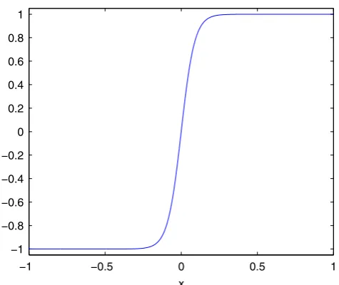
The gradient term in this energy is diffusive (‘philic,’represents weakly non-local interactions between the components that prefers complete mixing), while the second term is Ginzburg-Landau potential (repulsion potential,‘phobic,’prefers total separation of the phases). The competition between the two effects defines the profile ofjacross the interface (seeFigure 1for minimizer of W in one space dimension).
Now we combine the mixing energy with hydrodynamic kinetic energy, and write the energy law
d dt
Z r jð Þjuj2
2 dxþs 3e 2p Wffiffiffi2 ð Þj
" #
¼ 2D ½2
Heres is the interface surface tension constant (note that W tanh xffiffi 2
p
e
¼2pffiffi2
3e; xAℝ). Velocity u is taken to be
Onsager (1931b,a)the energy dissipation D (the quantity 2D is also called entropy production) should be proportional to some ‘rate’raised to a second power. Let us write it as a sum of viscous dissipation
1 4 Z
Z jð Þ∇uþ∇uTj2 dx
and dissipation on the interface
1 2 Z
j2〈M1ð ÞjðVuÞ;ðVuÞ〉dx
HereVis effective velocity of the phasefield
jtþ∇ðVjÞ ¼0 ½3
Note that this ensures conservation of the phasefieldj. Then we combine the variational Principle of Least Action (LAP) (Arnol'd, 1989) and Maximum Dissipation Principle (MDP) (Hyonet al., 2010). To apply LAP, we have to consider to separate independentflow maps related touandV. Writing the action functional
ℐ¼Z r jð Þjuj 2
2 dxs 3e 2p Wffiffiffi2 ð Þj
and applying the variation (in Lagrangian coordinates, with∇u¼0 constraint in thefirst case) we get
δℐ
δxu ¼ r jð ÞDtus 3e
2pffiffiffi2∇ ð∇j#∇jÞ ∇p;
δℐ
δxj¼ j∇m;
m¼s 3e
2pffiffiffi2 Djþ 1 e2 j
2 1
j
þr0ð Þj juj 2
2 : 8
> > > > > > > > < > > > > > > > > :
Here Dtj¼jtþu∇j is material derivative. Because of scale separation, for each variation in MDP we using only corre-sponding part of dissipation: viscous dissipation for variation with respect touand interface dissipation for variation with respect toV. The result we get is
ρðφÞDtuþσ 3ε
2pffiffiffi2∇⋅ð∇φ⊗∇φÞ þ∇p¼∇⋅ðηðφÞð∇uþ∇u TÞÞ
−φ∇μ¼φ2MðφÞðV−uÞ: 8
> < > :
−1 −0.5 0 0.5 1
−1 −0.8 −0.6 −0.4 −0.2 0 0.2 0.4 0.6 0.8 1
[image:3.612.185.423.57.257.2]x
Figure 1 Minimizer of energy (1),jð Þ ¼x tanh xffiffi
2 p
Combining this with [3] we get the Navier–Stokes/Cahn–Hilliard system:
Dtj¼∇ðMð Þj ∇ζÞ;
r jð ÞDtu¼ ∇pþ∇ðZ jð Þð∇uþ∇uTÞÞ s 3e
2pffiffiffi2∇ð∇j#∇jÞ; ∇u¼0;
m¼s 3e
2pffiffiffi2 Djþ 1 e2 j
2 1
j
þr0ð Þj juj 2
2 : 8
> > > > > > > > < > > > > > > > > :
½4
Remark 1: The sharp interface model assumes that the phases are subject to pure convection. Cahn-Hilliard equation is perturbation from that. Another way to perturb convection is Allen-Cahn equation, which is a gradientflow inj:
Dtj¼ mð Þjm
In the energy law this model would correspond to the following term related to dissipation on the interface:
1 2 Z
1 mð Þj Dtjj
2 dx
It is important to notice, that (unlike Cahn–Hilliard) this model does not have conservation ofj. But it does have other advantages (e.g., maximum principle, seeOnsager, 1931a,b).
Remark2: Consider the Oldroyd model for the incompressible viscoelasticfluid:
Ftþv∇F¼∇vF;
vtþv∇vþ∇p¼ZDvþ∇ðFFTÞ ∇v¼0:
8 > < > :
Under assumption that detF0¼1, we can claim thatF¼∇j(herejis a matrix), and rewrite the system as
jtþv∇j¼0;
vtþv∇vþ∇p¼ZDvþ∇ð∇j#∇jÞ; ∇v¼0;
8 > < > :
which is similar to the system [4] with no interface diffusion (M(j)¼0) [for more details seeLinet al., 2005).
Remark3: It is of certain interest to analyze sharp interface limit withe-0. SeeAbelset al. (2012)for an example of formal asymptotic analysis using inner and outer expansions.
2
Boundary Conditions
If we consider the energy law [2] on a bounded domainO, then integration by parts in both LAP and MDP will require boundary conditions
〈∇j;n〉¼0;
〈Mð Þj ∇ζ;n〉¼0; xA∂O; t40: u¼0:
8 > < > :
However,Qianet al. (2006)have shown that the model with energy dissipation at the solid boundary surface better matches molecular dynamics experiments, and avoids discrepancy of the contact line dynamics. More precisely, standard boundary conditions do not allow contact line to move along the boundary, while molecular dynamics experiments show, that near complete slip occurs in vicinity of contact line near the boundary.
Hence, we consider the following expression for energy dissipation (including bulk terms already mentioned above):
D ¼ 1
2 Z
O 1
2Z jð Þj∇uþ∇u
Tj2þj2〈M1ð ÞjðVuÞ;ðVuÞ〉
dxþ1 2 Z
∂O bju slip t j2þ
3e 2pffiffiffi2
s
gjjtþut∇tjj 2
dSx;
conditions onjand generalized Navier boundary conditions onu:
jtþut∇tjþg∂nj¼0; 〈Mð Þj∇ζ;n〉¼0;
buslip t
þZ jð Þ∂nð Þ ut s 3e
2pffiffiffi2∂nj∇tj¼0; un¼0; xA∂O; t40:
8 > > > < > > > :
Remark4: In generalized Navier boundary conditions the terms3e
2pffiffi2∂nj∂tjis the so-called uncompensated Young stress. See Qianet al. (2006)for expression in terms of contact angle and physical interpretation.
Remark5: The case above considers the equilibrium contact angle (De Genneset al., 2004;Rowlinson and Widom, 2002) to be p/2. For more general contact angleycQianet al. (2006)suggest boundary condition
jtþut∇tjþg∂nj¼0; 〈Mð Þj∇ζ;n〉¼0;
buslip t
þZ jð Þ∂nð Þ ut s 3e
2pffiffiffi2Lð Þj ∇tj¼0; un¼0; xA∂O; t40;
Lð Þ ¼j ∂njþ∂gfsð Þ=j ∂j; 8 > > > > > < > > > > > :
wheregfs¼ Cfs
2cosycsinðpj=2Þis an additional interfacial free energy density. The total energy considered in this case should be Z
O r jð Þjuj2
2 dxþs 3e
2pffiffiffi2 Wð Þ þj Z
∂OgfsdSx
3
Mixture of Three Fluids
Here we discuss several results for mixtures of more than two phases.
Kim and Lowengrub (2005) developed a thermodynamically consistent model for three-phaseflow, where they use con-centrations as a phase variables. However, they use mass-averaged velocity for the backgroundflow, which is quasi-incompressible (seeLowengrub and Truskinovsky, 1998;Abelset al., 2012).
Boyer and Lapuerta (2006);Boyeret al. (2010)build a model for three phaseflow using LAP with Lagrange multiplier tofind a chemical potentialsmfor each phase. They use volume averaged velocity to ensure incompressibility condition, which is preferable from numerical prospective. The phase part of the model they build is
ct¼M1Dζc; dt¼M2Dζd;
ζc¼ 3
4e∇ðS1∇cÞ þ 12
e ∂1Fð Þ þc b;
ζd¼ 3
4e∇ðS2∇dÞ þ 12
e ∂2Fð Þ þc b; b¼ S0
1
S1∂1Fð Þ þc 1
S2∂2Fð Þ þc 1 S3∂3Fð Þc
c¼〈c;d;1cd〉; S0¼ S11þS
1 2 þS
1 3
1
; M1S1¼M2S2¼M3S3¼M0: 8 > > > > > > > > > > > > > > > > < > > > > > > > > > > > > > > > > :
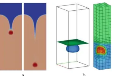
Boyeret al. show that Lagrange multiplier, mobility constraint and some additional requirements on repulsion potentialFare necessary to ensure energetic and dynamic consistency with a two-phase model in any combination (c0,d0,cþd1). Among other requirements, they ensure the third phase will not artificially appear in the region where only two phases are present. Authors confirm their analysis with numerical experiment (for example of implementation in 3D see inFigure 2(b)).
The Allen–Cahn/Navier–Stokes model by Brannick et al. (2015) was built using LAP and MDP for the case of constant (negligibly different) densities. Here authors use two labeling functions as a phase variables. The resulting system is
rðutþu∇uÞ þ∇p¼ ∇ ðlseþ2msvÞ
ftþu∇f¼ M1δ E
δf; ctþu∇c¼ M2
δE
where
δE
δf¼g1 e1∇
c1 2
2
∇f
" #
þe11 c1 2
2
f2 1
f
( )
δE
δc¼g2 e2Dcþ 1 e2 c21
c
þg1 c1
2 e1
2j∇fj 2þ 1
4e1 f21
2
;
se¼ g 1e1
c1 2
2
∇f#∇fg2e2∇c#∇c; sv¼ 1
2 ∇uþð∇uÞ T
h i
:
The authors analyze the model numerically in different configurations (Boussinesq approximation was used to incorporate gravity). Authors show analytically that the slip effect on the boundary of a solid may be introduced by a thin layer of nearly inviscidfluid (seeFigure 3), and qualitatively confirm this result with numerical experiment (seeFigure 2(a)).
References
Abels, H., Garcke, H., Grun, G., 2012. Thermodynamically consistent, frame indifferent diffuse interface models for incompressible two-phaseflows with different densities. Mathematical Models and Methods in Applied Sciences 22 (03), 1–39.
Ambravaneswaran, B., Wilkes, E.D., Basaran, O.A., 2002. Drop formation from a capillary tube: Comparison of one-dimensional and two-dimensional analyses and occurrence of satellite drops. Physics of Fluids (1994-present) 14 (8), 2606–2621.
Arnol'd, V.I., 1989. Mathematical methods of classical mechanics, vol. 60. Springer.
Aronson, I., 2014. Modeling crawling cell movement on soft engineered substrates. Soft Matter 10 (9), 1365–1373.
Boyer, F., 2002. A theoretical and numerical model for the study of incompressible mixtureflows. Computers & Fluids 31 (1), 41–68.
Boyer, F., Lapuerta, C., 2006. Study of a three component Cahn−Hilliardflow model. ESAIM: Mathematical Modelling and Numerical Analysis 40 (04), 653–687. Boyer, F., Lapuerta, C., Minjeaud, S., Piar, B., 2009. A local adaptive refinement method with multigrid preconditionning illustrated by multiphaseflows simulations..ESAIM:
Proceedings. EDP Sciences. pp. 15−53.
Boyer, F., Lapuerta, C., Minjeaud, S., Piar, B., Quintard, M., 2010. Cahn-Hilliard/Navier-Stokes model for the simulation of three-phaseflows. Transport in Porous Media 82 (3), 463–483.
Brannick, J., Liu, C., Qian, T., Sun, H., 2015. Diffuse Interface Methods for Multiple Phase Materials: An Energetic Variational Approach. Numerical Mathematics: Theory, Methods and Applications 8 (02), 220–236.
[image:6.612.218.406.59.184.2]Caginalp, G., 1986. An analysis of a phasefield model of a free boundary. Archive for Rational Mechanics and Analysis 92 (3), 205–245. Cahn, J.W., Hilliard, J.E., 1958. Free energy of a nonuniform system. I. Interfacial free energy. The Journal of Chemical Physics 28 (2), 258–267.
Figure 3 A schematic illustration offluid slip modeled by a fast variation of tangential velocity across a thin layer (diffuse interface) with a small viscositym.
[image:6.612.213.407.236.322.2]Chang, Y.-C., Hou, T., Merriman, B., Osher, S., 1996. A level set formulation of Eulerian interface capturing methods for incompressiblefluidflows. Journal of Computational Physics 124 (2), 449–464.
Cristini, V., Blawzdziewicz, J., Loewenberg, M., 1998. Drop breakup in three-dimensional viscousflows. Physics of Fluids (1994-present) 10 (8), 1781–1783. De Gennes, P.-G., Brochard-Wyart, F., Quere, D., 2004. Capillarity and Wetting Phenomena: Drops, Bubbles, Pearls, Waves. Springer Science & Business Media. Gao, M., Wang, X.-P., 2012. A gradient stable scheme for a phasefield model for the moving contact line problem. Journal of Computational Physics 231 (4), 1372–1386. Gao, M., Wang, X.-P., 2014. An efficient scheme for a phasefield model for the moving contact line problem with variable density and viscosity. Journal of Computational
Physics 272, 704–718.
Guillen-Gonzalez, F., Tierra, G., 2014. Splitting schemes for a Navier−Stokes−Cahn−Hilliard model for twofluids with different densities. JCM 32 (6), 643–664. Hohenberg, P.C., Halperin, B.I., 1977. Theory of dynamic critical phenomena. Reviews of Modern Physics 49 (3), 435.
Hooper, R., Toose, M., Macosko, C.W., Derby, J.J., 2001a. A comparison of boundary element andfinite element methods for modeling axisymmetric polymeric drop deformation. International Journal for Numerical Methods in Fluids 37 (7), 837–864.
Hooper, R.W., de Almeida, V.F., Macosko, C.W., Derby, J.J., 2001b. Transient polymeric drop extension and retraction in uniaxial extensionalflows. Journal of Non-Newtonian Fluid Mechanics 98 (2), 141–168.
Hu, H.H., Patankar, N.A., Zhu, M., 2001. Direct numerical simulations offluid-solid systems using the arbitrary Lagrangian-Eulerian technique. Journal of Computational Physics 169 (2), 427–462.
Hyon, Y., Kwak, D.Y., Liu, C., 2010. Energetic variational approach in complexfluids: Maximum dissipation principle. DCDS-A 24 (4), 1291–1304.
Kelly, D., Gago, D.S., Zienkiewicz, O., Babuska, I., 1983. A posteriori error analysis and adaptive processes in thefinite element method: Part I−Error analysis. International Journal for Numerical Methods in Engineering 19 (11), 1593–1619.
Kim, J., Kang, K., Lowengrub, J., 2004a. Conservative multigrid methods for Cahn−Hilliardfluids. Journal of Computational Physics 193 (2), 511–543.
Kim, J., Kang, K., Lowengrub, J., 2004b. Conservative multigrid methods for ternary Cahn-Hilliard systems. Communications in Mathematical Sciences 2 (1), 53–77. Kim, J., Lowengrub, J., 2005. Phasefield modeling and simulation of three-phaseflows. Interfaces and free boundaries 7 (4), 435.
Kim, S.J., Han, C.D., 2001. Finite element analysis of axisymmetric creeping motion of a deformable non-Newtonian drop in the entrance region of a cylindrical tube. Journal of Rheology (1978-present) 45 (6), 1279–1303.
Larson, R.G., 1999. The Structure and Rheology of Complex Fluids. New York: Oxford University Press.
Lee, H.G., Choi, J.-W., Kim, J., 2012. A practically unconditionally gradient stable scheme for the N-component Cahn-Hilliard system. Physica A: Statistical Mechanics and its Applications 391 (4), 1009–1019.
Li, J., Renardy, Y., 2000a. Numerical study offlows of two immiscible liquids at low Reynolds number. SIAM Review 42 (3), 417–439.
Li, J., Renardy, Y.Y., 2000b. Shear-induced rupturing of a viscous drop in a Bingham liquid. Journal of Non-Newtonian Fluid Mechanics 95 (2), 235–251. Lin, F.-H., Liu, C., Zhang, P., 2005. On hydrodynamics of viscoelasticfluids. Communications on Pure and Applied Mathematics 58 (11), 1437–1471.
Liu, C., Shen, J., 2003. A phasefield model for the mixture of two incompressiblefluids and its approximation by a Fourier-spectral method. Physica D: Nonlinear Phenomena 179 (3), 211–228.
Lowengrub, J., Truskinovsky, L., 1998. Quasi-incompressible Cahn−Hilliardfluids and topological transitions. Proceedings of the Royal Society of London. Series A: Mathematical, Physical and Engineering Sciences 454 (1978), 2617–2654.
National Materials Advisory Board, National Research Council, National Research Council, 1990. Liquid Crystalline Polymers. The National Academies Press. Onsager, L., 1931a. Reciprocal relations in irreversible processes. I. Physical Review 37 (4), 405.
Onsager, L., 1931b. Reciprocal relations in irreversible processes. II. Physical Review 38 (12), 2265.
Qian, T., Wang, X.-P., Sheng, P., 2003. Molecular scale contact line hydrodynamics of immiscibleflows. Physical Review E 68 (1), 016306. Qian, T., Wang, X.-P., Sheng, P., 2006. A variational approach to moving contact line hydrodynamics. Journal of Fluid Mechanics 564, 333–360.
Ramaswamy, S., Leal, L., 1999a. The deformation of a Newtonian drop in the uniaxial extensionalflow of a viscoelastic liquid. Journal of Non-Newtonian Fluid Mechanics 88 (1), 149–172.
Ramaswamy, S., Leal, L., 1999b. The deformation of a viscoelastic drop subjected to steady uniaxial extensionalflow of a Newtonianfluid. Journal of Non-Newtonian Fluid Mechanics 85 (2), 127–163.
Rowlinson, J.S., Widom, B., 2002. Molecular Theory of Capillarity. Mineola, N.Y: Dover Publications.
Sethian, J., Smereka, P., 2003. Level set methods forfluid interfaces. Annual Review of Fluid Mechanics 35 (1), 341–372.
Shen, J., 2011. Modeling and numerical approximation of two-phase incompressibleflows by a phase-field approach. Multiscale Modeling and Analysis for Materials Simulation. World Scientific. IMS, NUS, pp. 147−195..
Shin, J., Kim, S., Lee, D., Kim, J., 2013. A parallel multigrid method of the Cahn−Hilliard equation. Computational Materials Science 71, 89–96.
Tierra, G., Guillen-Gonzalez, F., 2014. Numerical methods for solving the Cahn−Hilliard equation and its applicability to related energy-based models. Archives of Computational Methods in Engineering. 1–21.
Toose, E., Geurts, B., Kuerten, J., 1995. A boundary integral method for two-dimensional (non)-Newtonian drops in slow viscousflow. Journal of Non-Newtonian Fluid Mechanics 60 (2), 129–154.
Unverdi, S.O., Tryggvason, G., 1992. A front-tracking method for viscous, incompressible, multi-fluidflows. Journal of Computational Physics 100 (1), 25–37. Utracki, L., Favis, B., 1989. Polymer Alloys and Blends, vol. 4. New York: Marcel Dekker.
van der Waals, J., 1979. The thermodynamic theory of capillarity under the hypothesis of a continuous variation of density. Journal of Statistical Physics 20 (2), 200–244. West, J.L., 1990. Polymer-Dispersed Liquid Crystals. In: Weiss, R.A., Ober, C.K. (Eds.), Liquid-Crystalline Polymers, Chapter 32, vol. 435 of ACS Symposium Series. ACS
Publications, pp. 475–495.
Wheeler, A., Boettinger, W., McFadden, G., 1992. Phase-field model for isothermal phase transitions in binary alloys. Physical Review A 45 (10), 7424. Yue, P., Feng, J.J., Liu, C., Shen, J., 2004. A diffuse-interface method for simulating two-phaseflows of complexfluids. Journal of Fluid Mechanics 515, 293–317. Zheng, L., Zhang, H., 2000. An adaptive level set method for moving-boundary problems: application to droplet spreading and solidification. Numerical Heat Transfer: Part B: