Abstract
It is usually discovered in the data collection phase of a survey that some units in the sample are ineligible even if the frame information has indicated otherwise. For example, in many business surveys a nonnegligible proportion of the sampled units will have ceased trading since the latest update of the frame. This information may be fed back to the frame and used in subsequent surveys, thereby making forthcoming samples more efficient by avoiding sampling nonnegligible units. We investigate what effect on survey estimation the process of feeding back information on ineligibility may have, and derive an expression for the bias that can occur as a result of feeding back. The focus is on estimation of the total using the common expansion estimator. We obtain an estimator that is nearly unbiased in the presence of feed back. This estimator relies on consistent estimates of the number of eligible and ineligible units in the population being available.
SSRC Methodology Working Paper M03/01
Feeding back Information on Ineligibility from Sample Surveys to the
Frame
Feeding back information on ineligibility from sample surveys to
the frame
DAN HEDLIN1 and SUOJIN WANG2
ABSTRACT
It is usually discovered in the data collection phase of a survey that some units in the sample are ineligible even if the frame informatio n has indicated otherwise. For example, in many business surveys a nonnegligible proportion of the sampled units will have ceased trading since the latest update of the frame. This information may be fed back to the frame and used in subsequent surveys, thereby making forthcoming samples more efficient by avoiding sampling nonnegligible units. We investigate what effect on survey estimation the process of feeding back information on ineligibility may have, and derive an expression for the bias that can occur as a result of feeding back. The focus is on estimation of the total using the common expansion estimator. We obtain an estimator that is nearly unbiased in the presence of feed back. This estimator relies on consistent estimates of the number of eligible and ineligible units in the population being available.
KEY WORDS: dead unit, feed back bias, overcoverage, permanent random number sampling, panel survey, co-ordinated samples.
1
University of Southampton, Department of Social Statistics, Southampton SO17 1BJ, UK. e-mail: [email protected]
1. INTRODUCTION
To facilitate estimation of change, consecutive samples in a repeated survey are usually overlapping. If several surveys draw samples from the same frame, it is often desirable to spread the response burden out by making sure that samples for different surveys are not overlapping to a greater extent than necessary. This is particularly desirable if the frame is moderately large and used for many continuing surveys, which is a situation that many national statistical institutes face when conducting business surveys. Stratified simple random sampling is a very common design for business surveys. The skewed distribution of businesses calls for large sampling fractions in many strata, which aggravates the response burden for medium size and large businesses. Both estimation of change and response burden issues are of paramount importance in official business statistics. Therefore, sampling systems have been constructed that allow the organisation to co-ordinate samples, either positively or negatively (i.e. to create overlap or to make sure that there is little overlap).
predetermined sample size n, a point is selected (randomly or purposively) on the PRN line and the n units to the right (say) are included in the sample. Two srswors are fully co-ordinated if they are drawn from the same interval. For overviews and further details see Ohlsson (1995) and Ernst, Valliant and Casady (2000). Table 1 shows starting points of sampling intervals of some of the business surveys the ONS conducts on a regular basis.
[Table 1 about here]
Samples for repeated surveys can also be selected with a panel technique where a set of rotation groups are selected at the first wave and one, say, of the groups is replaced with a fresh rotation group at the second wave and the other groups are retained in the sample. The difference between PRN sampling and panel sampling is more about the way to control overlaps than having different sampling designs.
for repeated surveys. This is in principle how information of dead units is treated in business surveys at the ONS and some other national statistical institutes.
It would seem natural that this new information should be made available to other sample surveys, which otherwise may include the dead units in their samples and therefore lose precision. However, as pointed out by Srinath (1987) among others, such a procedure may cause bias. We refer to this as feed back bias, which results whenever the sampling mechanism is not independent of the feed back procedure. For example, consider a situation where all dead units are found and deleted at the first wave of a panel survey. If no further deaths have occurred up to the second-wave observation of the panel units, the second-wave sample contains only live units. Without knowledge of the total number of live units in the population at the time of the second wave, an unbiased estimator of the total cannot be constructed. While more information about the population has been gathered when the deaths were recorded at the first wave, there is actually less information in the second wave-sample on the proportion of live units in the population.
dead units in the rotating sample of the Survey of Employment, Payroll and Hours conducted by Statistics Canada. Hidiroglou and Laniel (2001) discuss the feed back issue briefly. A general discussion of frame issues is given by Colledge (1995) and overviews of issues associated with continuing business surveys include College (1989), Hidiroglou and Srinath (1993), Srinath and Carpenter (1995), and Hidiroglou and Laniel (2001).
Instead of the terms eligible and ineligible we use the more emotive words dead and live, although our reasoning does cover all kinds of ineligibility. We confine our discussion to
the estimation of the total of some study variable y′=
(
y1,y2,...,yN)
on a population Uwith unit labels
{
1,2,...,N}
,∑
=
U k
y y
τ . ( 1 )
When the sampled units are observed, we assume that all dead units in the sample are classified as dead and the frame is updated with this information. This may be difficult in practice. In some surveys, however, the eligibility of all nonresponding units can be correctly identified.
2. AN EXPRESSION FOR FEED BACK BIAS
We assume throughout that a dead unit is always out of scope and that the value of the study variable of a dead unit is always zero. (It is conceivable that dead units are eligible in some surveys; for example, a business survey collecting data on production may have defined businesses that were alive at least a part of the reference period as eligible.) We adopt the design-based view that the survey population and the study variable are fixed and non-stochastic at any given point in time. The situation we address is as follows. One or more samples are drawn from the frame which comprises the original survey population, Uorig. For convenience we assume that the frame units and population units
are of the same type. We refer to the updated frame, where all dead units that have been included in samples from Uorig have been excluded, as the current survey population,
Ucurrent. For example, two surveys may simultaneously work with a sample each, and
after they have fed back, Uorig has shrunk to Ucurrent. We disregard births of new units and
other deaths than those deleted through samples from Uorig. We will also disregard
Let Ud and Ul be the two subsets of the current survey population, Ucurrent = Ud ∪Ul,
that consist of dead and live units, respectively. A unit flagged on the frame as live belongs to either Ud and Ul. Units that are flagged as dead but for which the
independence of detection and the sampling mechanism cannot be assured are called dead by sample survey sources. In our set- up, these are the dead units detected in samples taken from Uorig. Let the set of these units be denoted by Usd, and we have the
relationship Uorig =Ucurrent∪Usd. Let N with a proper subscript be the size of each
population, respectively. Then Ncurrent = Nl+ Nd, and Norig = Nl+ Nd + Nsd. At the time
when samples are drawn from Ucurrent, Ncurrent and Nsd are known numbers, whereas Nl
and Nd are unknown. Moreover, Nsd, Nd and Ncurrent could be viewed as random
depending on feed back results, while Nl is fixed. Following principles of Durbin (1969)
and more recently in Thompson (1997), we would in many situations prefer to condition on Nsd. For example, if it is seen at the time when a sample is taken from Ucurrent that Usd
is in fact empty, then it does not seem appropriate to include in the inference the poss ibility that Nsd could have been large. However, to analyse the development of the
feed back bias over a series of waves in a forthcoming panel survey, unconditional analysis would be preferable. We also provide an expression for the unconditional feed back bias.
[Figure 1 about here]
Denote by Unodeads the part of Ucurrentthat was covered by the previous sample(s) drawn
from Uorig; see Figure 1. Clearly, Unodeads is a random set depending on previous samples.
Since Unodeads is winnowed from dead units we have Unodeads⊂Ul. The complement to
of Ul. We have Unodeads∪Uwithdeads =Ul∪Ud= Ucurrent. To derive the feed-back bias
we will consider a sample of size n with a sample part sa of size na taken from Unodeads
through PRN sampling or a panel sampling technique, and the remaining part sb is taken
from Uwithdeads. Let I
(
k∈sa)
=1 when unit k is included in sa, otherwise I(
k∈sa)
=0.Recall that yk =0 if k is a dead unit. Thus we have
∑
sayk =∑
UlykI(
k∈sa)
=∑
UcurrentykI(
k∈sa)
and, assuming that Nl > 0,[
]
l a sd a N n N alive k sk∈ | , =
Pr . The probability is conditional on unit k being alive since it is
determined by design that only live units can be included in Unodeads. Denote the bias of
an estimator θˆ for the parameter θ by B
( )
θˆ,θ . Then with respect to the population totalk U y =Σ currenty
τ , the bias of a general linear estimator =
∑
a a
s k k s
y w y
tˆ( ) , with any given
k w ’s, is
(
)
{
[
]
}
kl a k U k
U k a sd
sd y s y y N n w y N alive k s k E w N t B l l a − Σ = − ∈
=
∑
| , 1 1, ˆ( ) τ
=
∑
− current U k l a k y N n w1 . ( 2 )
In particular, the bias of the expansion estimator =
∑
a a s k a current s y y n N ) ( ˆ
τ is
(
y sd)
s
y N
Bτˆ( a),τ = y l d
N N
τ . ( 3 )
Alternatively, sampling of sa can be seen as a two-phase sampling scheme. Note that in
the first phase,
[
k Unodeads kalive,Nsd]
orig l orig nodeads N N N N = l nodeads N N
= . ( 4 )
Thus,
[
]
l a nodeads a l nodeads sd a N n N n N N N k sk∈ alive, = =
Pr . ( 5 )
Note that Nnodeads (and thus Nsd) cancels out. The probability of
(
k∈sa)
depends on thefeed back process to have taken place but not on the size of Usd.
Next, to derive the bias for the sample part sb of size nb taken from Uwithdeads, first note
that
(
k∈Uwithdeads)
is the same event as(
k∉Up)
, where Up =Unodeads∪Usd is the partof Uorig covered by previous samples. Then
[
k Uwithdeads Nsd]
Pr ∈
[
]
orig withdeads orig p orig sd p N N N N N N U
k∉ = − =
=Pr . ( 6 )
This conditional probability again does not depend on the relative sizes of Unodeads and
Usd. On the other hand, the probability of including a unit in sb given that feed back has
occurred is
[
]
. Pr withdeads b sd b N n N sk∈ = ( 7 )
From ( 7 ) we obtain that the conditional expected value of =
∑
b b
s k k s
y w y
tˆ( ) is
(
sd)
=s
y N
t
E ˆ( b) E
∑
U k k sd withdeadsb w y N
N n withdeads = withdeads b N n l nodeads l N N N −
∑
Uorig k ky
The second equation above is due to the fact that givenNsd, all Nl live units in Uorig are
equally likely to be in Uwithdeads, which has Nl−Nnodeads live units. Therefore, the
conditional bias of ˆ(sb) y t is
(
y sd)
=s
y N
t
Bˆ(b),τ
∑
− − orig U k l nodeads l withdeads b k y N N N N n w 1
∑
− − = current U k l nodeads l withdeads b k y N N N N n w1 . ( 8 )
For the expansion estimator ( )sb y
τˆ with weights wk = Ncurrent nb the bias is
(
y sd)
= sy N
t B ˆ( b),τ
y
Bτ , ( 9 )
where 1 − − = l nodeads l withdeads current N N N N N
B
(
)
(
)
l withdeads nodeads current l nodeads l current N N N N N N N
N − − −
= withdeads l nodeads d N N N N − =
(
)
(
orig p)
l sd p d N N N N N N − − − = .
The bias is always non-positive since B≤0. It is easy to see that B is an increasing
function of Nsd since Nd = Ntotaldeads−Nsd, where Ntotaldeads is the fixed number of all
dead units in Uorig. It is also readily seen that the maximum of B is attained when Usd
encompasses all dead units in Uorig, that is, when Nsd = Ntotaldeads.
Combining ( 9 ) with ( 3 ) we obtain the overall bias of s k current y y n N current Σ =
τˆ to be
(
y y Nsd)
=Bτˆ ,τ E(τˆy |Nsd)−τy = y
withdeads nodeads b a l d N N n n n n N N τ − y
c~τ
The bias in the expansion estimator is really down to not knowing the correct population size. In ( 3 ) the bias stems from multiplying the sample average over live units with Ncurrent rather than the unknown Nl. The bias from the sample parts sa and sb will in
absolute terms be less than ( 3 ) and ( 9 ), respectively, if some of the dead units in the samples from Uorig have not been identified as dead and therefore have not been weeded
out. This would happen, for example, if the status of nonresponding units is difficult to determine.
An unconditional analysis in the presence of feed back can be obtained directly by taking
expectation of ( 10 ) with respect to Nsd. Thus, unconditionally, we have
y s k current current y n N
E −τ
∑
=
( )
( )
ywithdeads l b withdeads sd p b a l sd totaldeads N nN n N N E N n n n n N N E N τ − − − − y cτ
= , ( 11 )
where E
( )
Nsd = NpNtotaldeads Norig.Lavallée (1996) took an interesting approach to a similar problem with panel survey data. In that paper, the problem of frame update using panel with rotation is addressed among other issues. Our approach is different from the approach of that paper in that we consider
3. THREE SIMPLE STRATEGIES AND A SIMULATION STUDY
A strategy, which is referred to as Strategy 1 here, is to feed back, delete the set Usd from
the frame and accept the feed back bias. However, the size of the bias is seldom known.
The estimator for Strategy 1 is =
∑
current s k current y y n N
τˆ where scurrent is a sample taken
from Ucurrent. To obtain Strategy 2, note that if consistent estimates of Nd and Nl are
available these may be plugged into ( 10 ) or ( 11 ) and an estimator with favourable properties is obtained:
(
ˆ)
11 ˆ
ˆy′ =τy +c −
τ , ( 12 )
where
− − − = p orig sd p b a l d N N N N n n n n N N c ˆ ˆ
ˆ for both the conditional and unconditional cases
since the term nb
(
nNlNwithdeads)
−1 in ( 11 ) is negligible. The estimates Nˆ and d Nˆ of the lsizes of the domains Ud and Ul can be obtained from a sample from the original or
current survey population with
( )
∈ = otherwise. 0, , unit if ,1 d l
k
N N k y
As the following argument shows, we do not expect the bias of ( 12 ) to be large:
(
)
[
1]
( )
(
)
11 ˆ ˆ
1
ˆ + − ≈ + −
=
′ E c E c
E τy τy τy =τy
(
1+c)(
1+c)
−1 =τy.precision will suffer as part of the sample is lost on ineligible units. The estimator of
Strategy 3 is ″=
∑
orig
s k orig
y y
n N
τˆ .
A simulation study may shed some light on which of the Strategies 1-3 is to be preferred. Natural measures for comparing the strategies are bias and variance. In business surveys, estimates for subpopulations (industries) are often more interesting than the whole population. To simulate a subpopulation, a frame consisting of 1000 units was created to form the original survey population. A gamma distributed value, Y1, was associated with each unit. We used the same gamma distribution as the one that generated Population 12 in Lee, Rancourt, and Särndal (1994, p. 236). The coefficient of variation (population standard deviation divided by the mean) was 0.57. Another study variable, Y2, was created by performing independent Bernoulli trials, one for each population unit, which obtained value 1 with probability equal to 0.5 and value 0 otherwise. Unlike in Lee, et al., some of the units were dead. Each unit was independently of other units classified as dead with a probab ility Pdead. All dead units were assigned zero values for both Y1 and
Y2. A set of Y1 and Y2 were simulated for each of four values of Pdead: 0.03, 0.05, 0.2,
and 0.5. These sets contained 29, 54, 201 and 494 dead units, respectively.
A PRN was attached to each unit and the units were laid out along a PRN line. The first sample, s1, was drawn by identifying the 500 units with the smallest PRNs. All dead units in s1 were flagged as ‘dead by sample survey sources’. Hence, Up covered approximately
in Strategy 2 were based on s1. A second sample, denoted by s2current, was drawn by
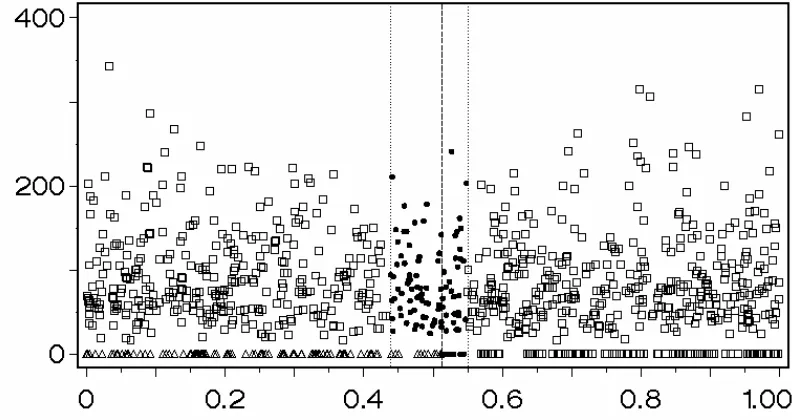
taking 100 units to the right of a starting point, start 2, disregarding units dead by sample survey sources. Another sample of 100 units was selected from start 2, but units dead by sample survey sources were this time allowed to be included in this sample. He nce, this sample was drawn from Uorig, and we denote it by s2orig. Figure 2 shows the PRN
intervals and the study variable Y1.
[Figure 2 about here]
The procedure described in the preceding paragraph was repeated 1000 times. That is, for each of the values of Pdead mentioned above and for each of three starting points of s2, to
be defined, 1000 sets of PRNs were generated and attached to the units. The frame was reordered for each new set of PRNs, and three samples were drawn for each reordering (s1, s2current, and s2orig). Two values of start 2, 0.0 and 0.7, were chosen so as to make the
proportion of s2current that fell in Unodead 100% and 0%, respectively. That is, na/n was set
to 100% and 0%. Further, to make na/n on average 50% under each of the chosen Pdead,
appropriate values of start 2 were derived. They are 0.448, 0.447, 0.438, and 0.4 for the Pdead values 0.03, 0.05, 0.2, and 0.5, respectively.
In summary, the population and samples sizes, the study variables Y1 and Y2, and which of the units tha t were dead were held fixed in our study. For twelve combinations of Pdead
and na/n, the reordering of the units on the PRN line through the simulation of new PRNs
made the following factors vary:
§ which of the units that were included in s1, s2current, and s2orig;
§ which of the units that belonged to Unodeads and Uwithdeads.
Thus the quantities Nsd, Nd and Ncurrent vary in the simulations. It seems practical to let
them do so rather than to control them in an experiment with more factors than Pdead and
na/n.
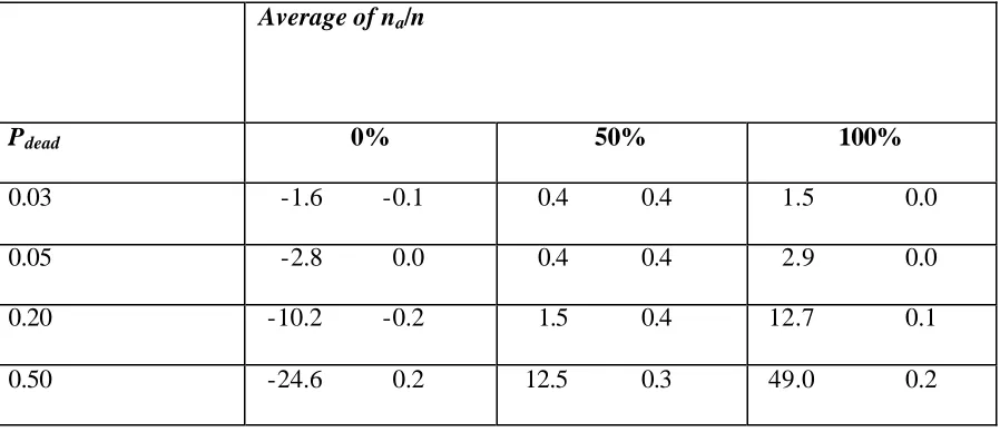
Table 2 shows the empirical relative bias of Strategies 1 and 2, computed as the straight average of the 1000 differences between the estimate and the parameter in terms of the percentage of the total obtained in the simulation. Strategy 3 is unbiased and is therefore not included in Table 2. The bias of Strategy 3 that nevertheless appeared in the simulations reflects the simulation error; it was at most 0.5%. As seen in Table 2, Strategy 2 is virtually unbiased as well. Note that the simulated bias under Strategy 1 is what ( 11 ) predicts (with allowance for simulation error). This bias is appreciable in nearly all cases and if the proportion of dead (or ineligible) units is high the bias can be very severe indeed. Table 3 shows the empirical coverage probabilities. While Strategy 2 gives in all cells coverage probabilities close to the targeted 95%, Strategy 1 achieves that in general only for the population with 3% dead units. The coverage probability under Strategy 1 tends also to be acceptable for populations with a larger proportion of dead units, if half of the sample is taken from the part of the PRN line where dead units have been weeded out, and the other half from the part of the PRN line where the original proportion of dead units has been retained, as the negative bias from the first half of the sample tends to cancel out the positive bias from the second half.
[Table 2 about here]
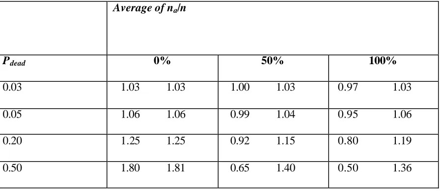
The variance of the simulated estimates was computed. Tables 4 and 5 show the variance of Y1 and Y2, respectively, under Strategies 2 and 3 relative to that of Strategy 1, which in all cases gives a smaller variance than Strategy 3. Hence, considering the extra complexity of Strategy 2, the feed back strategy seems preferable for populations with a small proportion of ineligible units, say 3% or less. If this proportion is larger than, say, 5%, the bias of Strategy 1 may cause poor coverage probabilities and misleading
estimates. The variance of Strategy 2 is no worse than that of Strategy 3; in most cases Strategy 2 is superior. The non- monotone variance ratios in the bottom row of Table 4 is due to the estimation of Nd and Nl combined with the specific details of the simulation.
[Table 4 about here]
[Table 5 about here]
4. DISCUSSION
This paper gives conditional and unconditional expressions for the feed back bias when the total is estimated with the common expansion estimator. We have shown that the feed back bias can be large. With as little as 5% ineligible units on the frame, feeding back information of these from sample surveys can result in about 2-3% bias. However, a small-scale simulation study indicates that if the proportion of ineligible units is 3% or less, the feed back strategy does not seem to create problems in terms of bias and variance.
retaining ineligible unit on the frame and letting them be included in further samples. This estimator relies on the availability of consistent estimates of the number of eligible and ineligible units in the population. These estimates may be obtained from an earlier sample in which the unbiased strategy of letting units that have been found dead be included in the sample.
In order to facilitate the theoretical development, we have made simplifying assumptions. The most important of these is the assumption that all dead units have been found in earlier sample surveys and have been fed back to the frame. We have envisaged a frame with one ‘white’ area, where all ineligibles have been flagged as such, and one ‘black’ area, where no ineligibles have been touched. In practice, this is not likely to happen. If the frame is moderately large and used for many continuing surveys, some of which may feed back to varying intensity, the frame will turn ‘grey’ rather than ‘black and white’. Clearly, the feed back bias will then be less severe than in the ‘black and white’ situation. It has not, however, been in the scope of this paper to quantify the bias for a ‘realistically grey’ frame. In this sense, what has been examined in this paper is a worst case scenario.
ACKNOWLEDGMENT
REFERENCES
COLLEDGE, M.J. (1989). Coverage and Classification Maintenance Issues in Economic Surveys. In Panel Surveys. (Eds. Kasprzyk, D., Duncan, G. J., Kalton, G., and Singh, M. P.). New York : Wiley, 80-107.
COLLEDGE, M.J. (1995). Frames and Business Registers: An Overview. In Business Survey Methods. (Eds. Cox, B., Binder, D., Chinappa, N., Christianson, A., Colledge, M. and Kott, P). New York: Wiley, 21-47.
DURBIN, J. (1969). Inferential Aspects of the Randomness of Sample Size in Survey Sampling. In New Developments in Survey Sampling. (Eds. Johnson, N.L. and Smith, H.). New York: Wiley, 629-651.
ERNST, L.R., VALLIANT, R., and CASADY, R.J. (2000). Permanent and Collocated Random Number Sampling and the Coverage of Births and Deaths. Journal of Official Statistics, 16, 211-228.
HIDIROGLOU, M.A. and LANIEL, N. (2001). Sampling and Estimation Issues for Annual and Sub-Annual Canadian Business Surveys. International Statistical Review. 69, 487-504.
HIDIROGLOU, M.A. and SRINATH, K.P. (1993). Problems Associated with Designing Subannual Business Surveys. Journal of Business and Economic Statistics, 11, 397-406.
LAVALLÉE, P. (1996). Frame Update Problems with Panel Surveys. Proceedings of Statistical Days ’96, Statistical Society of Slovenia, 252-261.
OHLSSON, E. (1995). Coordination of Samples Using Permanent Random Numbers. In Business Survey Methods. (Eds. Cox, B., Binder, D., Chinappa, N., Christianson, A., Colledge, M. and Kott, P). New York: Wiley, 153-169.
SCHIOPU-KRATINA, I. and SRINATH, K.P. (1991). Sample Rotation and Estimation in the Survey of Employment, Payrolls and Hours. Survey Methodology, 17, 79-90.
SRINATH, K.P. (1987). Methodological Problems in Designing Continuous Business Surveys: Some Canadian Experiences. Journal of Official Statistics, 3, 283-288.
SRINATH, K.P. and CARPENTER, R.M. (1995). Sampling Methods for Repeated Business Surveys. In Business Survey Methods. (Eds. Cox, B., Binder, D., Chinappa, N., Christianson, A., Colledge, M. and Kott, P). New York: Wiley, 171-183.
Table 1. Starting points of the PRN sampling intervals of some of the business
surveys the UK Office for National Statistics conducts
Survey Starting point
of sampling interval
The Monthly Inquiry for the Distribution and Services Sector, and other monthly surveys covering other sectors of the business population
0
The Quarterly Capital Expenditure Inquiry 0.125
The UK Survey of Products of the European Community
0.375
The Inquiry of Stocks 0.5
Table 2. Bias, % of total of Y1. The first entry in each cell is the bias under Strategy
1, the second is the bias under Strategy 2
Average of na/n
Pdead 0% 50% 100%
0.03 -1.6 -0.1 0.4 0.4 1.5 0.0
0.05 -2.8 0.0 0.4 0.4 2.9 0.0
0.20 -10.2 -0.2 1.5 0.4 12.7 0.1
0.50 -24.6 0.2 12.5 0.3 49.0 0.2
Table 3. The coverage probability in percentage for estimating total of Y1. The first
entry in each cell is the under Strategy 1, the second is the coverage probability
under Strategy 2.
Average of na/n
Pdead 0% 50% 100%
0.03 94.6 94.3 94.6 94.8 94.3 95.1
0.05 93.3 95.2 94.4 93.9 90.8 95.0
0.20 65.9 94.5 93.8 94.8 46.1 94.6
[image:22.596.83.533.508.705.2]Table 4. Variance ratio of the estimator of the total of Y1. The first entry in each cell
is the variance under Strategy 2 relative to that of Strategy 1, the second is the
variance under Strategy 3 relative to Strategy 1.
Average of na/n
Pdead 0% 50% 100%
0.03 1.04 1.04 1.00 1.06 0.98 1.08
0.05 1.08 1.08 0.98 1.14 0.95 1.15
0.20 1.28 1.28 0.85 1.27 0.83 1.46
[image:23.596.85.534.535.730.2]0.50 1.85 1.85 0.52 1.34 0.58 2.24
Table 5. Variance ratio of the estimator of the total of Y2. The first entry in each cell
is the variance under Strategy 2 relative to that of Strategy 1, the second is the
variance under Strategy 3 relative to Strategy 1.
Average of na/n
Pdead 0% 50% 100%
0.03 1.03 1.03 1.00 1.03 0.97 1.03
0.05 1.06 1.06 0.99 1.04 0.95 1.06
0.20 1.25 1.25 0.92 1.15 0.80 1.19
Figure 1. The original survey population, Uorig, and its subsets.
Figure 2. A plot of one of the simulated populations, the study variable Y1 against
the PRNs, with Pdead = 0.20. The dots are units included in s2current (the sample from
the current survey population); the triangles are units that are dead by statistical
sources and squares represent units belonging to the current survey population but
are not included in the sample from this population. The PRN interval for s1 (the
500 units in the first sample from the original survey population) is (0, 0.51) and the
one for s2current is (0.44, 0.55).
sb
Uwithdeads
Usd
Unodeads
sa