The Economic Specification o f the Neoclassical
Production Function — a case study
M I C E A L ROSS
A production function may be defined as the mathematical expression o f the technological information which relates the quantities o f inputs to quantities o f outputs. As such, the concept is perfectly general and a specific function may be given as a single point, a set o f points, a single continuous or discontinuous function, or a system o f equations. The neoclassical production function is essentially a single continuous function with continuous first and second order partial deriva tives or a system o f such equations. Addressing itself directly to marginal analysis and the neoclassical function this paper excludes consideration o f other functions of major importance in economic analysis. Foremost among these are the linear and point functions which underlie most o f the studies involving linear pro gramming and game theory and the fixed proportions functions used in Input-Output analysis.
In neoclassical theory, as formulated by Hicks and others,1 the firm's decision
makers are assumed to possess two sets o f data: first, complete knowledge o f the production technology available to them and second, product demand informa tion. The first assumption implies that a given production process has some "true" functional representation, perhaps o f a stochastic nature, which involves some definite set o f variables either in a single equation or a set o f equations and that this underlying relationship is known. Given the assumptions o f profit maximisation and rationality the economic implications follow as simple mathematical tautologies for any given price conditions.2
However in real world situations this ideal so seldom, i f ever, obtains that some economists have come to regard the neoclassical production model as completely non-operational3 as an analytical tool for studying the behaviour o f the complex
technology o f the modern production process. They point to empirical research 1. An excellent brief statement of the Hicksian production function and its underlying assump tions is presented in T . H . Naylor and J . M . Vernon, Microeconomics and decision models of the firm, New York, 1970, pp.
7°~73-2. M . Ross, "Some management aspects of production functions", to be submitted to the Irish Journal of Agricultural Economics and Rural Sociology.
3. T . H . Naylor and J. M . Vernon, op. cit., p. 87; also M . Shubik, "A curmudgeon's guide to Microeconomics", Review of Economic Literature, Vol. VIII, No. 2, 1970, p. 411.
to justify their pessimism.4 Here it is usually found that the economic, physical
and biological logic underlying the function is largely unknown, as is the logic o f entrepreneurial decision-making within a complex business organisation. In such a situation the economist w i l l hypothesise that the function can be approximated by some given algebraic form, with several unknown parameters to be estimated from the available data. The chief difficulty with this procedure is that the economic inferences which are drawn from the estimated parameters often depend critically upon the algebraic form chosen. It frequently happens that alternative forms fit the data equally well but have very different implications for the most profitable level o f inputs. Clearly, where the basic logic is only hypothesised there is the further danger that relevant variables and relationships will be omitted through ignorance; and biassed estimates of the structure of the process, and its response to price situations, obtained.
Even i f the basic logic were known with certainty, the empirical construction of a model will frequently require a compromise between what is computationally feasible and what is theoretically desirable. For instance; some o f the variables, known to be relevant, may be unobservable. Again, data* availability and estima tion resources may limit the number o f separate variables that can be considered. In addition, the functional relationship to' be fitted needs to be manageable, both in terms of estimation and of testing. Often a worthwhile compromise may not be possible. Neoclassical theory assumes furthermore that the entrepreneur possesses full knowledge o f product demand information as well ;as advance information on the level o f inputs not under his control (e.g. weather, genetic make-up). Empirical applications are typically characterised by risk and uncertainty. Prices have to be forecast, and the levels o f uncontrollable inputs predicted. The degree of risk and uncertainty involved w i l l indicate whether a marginal analysis approach
is warranted. , As mentioned earlier, where production logic is unknown the form of equation
selected automatically imposes certain constraints on the' basic relationships and implies the economic optima. I f the margins of error in predicting price and output levels are likely to be considerable, it has been argued, the selection of an equation may compound the difficulties. Hildreth5 suggested1 that a procedure which
obtains maximum likelihood estimates o f discrete points on the production function may be preferable under these conditions.
Again, there are limits to the mathematical procedures for optimising continuous functions, assuming that all equations are indeed continuous. I f the model embraces complex choice or allocation problems linear programming or related approaches are probably most appropriate in determining optimum levels o f inputs and output; and these should be used in preference to continuous functions.6
i
4. The interested reader is referred to T . H . Naylor and J . M . Veriion, op. cit., pp. 132 et seq., for a more complete statement. J
5. G. C . Hildreth, "Point estimates of ordiiiates of concave functions," Journal of the American Statistical Association, Vol. 49, 1954. I
I f there is considerable output and price uncertainty these alternative approaches may be not only computationally simpler, but also o f sufficient accuracy for decision-making purposes.
This paper takes the view that these objections have considerable validity. Accordingly, the problems o f the economic specification are considered in a context where the neoclassical model is most likely to be operational, i.e., the data are derived from scientific experiment, the model is relatively simple, and the time-lags between input and output are sufficiently short to enable reasonable forecasts of prices to be made. Although the focus in this studyis on production functions, most o f the discussion applies with equal force to other neoclassical models (cf. Prais's discussion o f demand relations, or Pratschke's specification o f Engel functions).7 Similarly, the illustrative material's base in agriculture does
not mean that the analysis is not equally valid in other industrial contexts. Greater data availability has made agriculture a rich source o f examples, as the perusal o f any econometric textbook w i l l substantiate.
The Experiment
Except where instigated by an economist very few scientific experiments seek to define continuous production functions—or response curves.8 The case study
presented here was unusual in that the experiment proved amenable to such analysis.9 This Danish experiment1 0 sought to determine the effect o f varying
levels o f protein and energy rations on the performance o f fattening pigs from weaners (44 lb.) to market weight (198 lb.).
The protein, derived mainly from skim milk and a protein-rich mixture (two parts soyabean meal, and one part meat and bone meal)1 1, was fed as a constant
level at one o f the three following levels:—
Low Normal High
Skim milk (lb.) 1-65 3-3 4-63
Protein mix (oz.) 1-94 3-8 5*47
The fixed daily quantity o f barley was stepped up after every 11 lb. o f the pig's growth. Each increase was designed to cater for the increasing requirements of the
7. S.J. Prais, "Non-linear estimation of the Engel curves", Review of Economic Studies, Vol. 20, 1953; also J. L . Pratschke, Income-Expenditure Relations in Ireland ig6s-ig66. Dublin: Economic and Social Research Institute. Paper No. 50, 1969.
8. It may be confusing that what are essentially regression lines to the statistician takes on differ ent names in different applications and in different disciplines e.g. production functions, engel-, cost-, demand-, supply curves to the economist, response curves to the agronomist, reaction equations to the chemist etc.
9. E . Vestergaard Jensen, "Forskellige protein og fodernormer til svin i driftsokonomisk belysning", Tolvmandsbladet Nr. 1, Copenhagen, 1958.
10. H . Clausen, "Forsog SV 698 Sj. n " , Bilag til oversikten, Forsogslaboratoriets efterarsmode, Copenhagen, 1956.
growing animal, and was at a rate calculated to maintain the pig on the required (stepped) feeding plane. The five feeding planes ranged from an average intake of 3*6 fodder units (f.u.) per day, up to 6-0 f.u. The barley was added to the fixed
I
TABLE
I :
Descriptions of Main Aspects of Treatments. i Percentage Protein in
Per pig daily the ration at
Treatment Intensity of Protein 1
Protein Number Feeding Standard Total
1
Protein Feeding
f.u. average f.u. fixed 44 lbs 198 lbs
i Weak low 3-64 •41 1 1 7 7 7
2 Weak normal 3-77 •82 17-0 8-8
3 Weak high 3-72
I-IJ*
18-5 9 74 Moderate low 4-17 •41' 10-5 7-6
5 Moderate normal 4*21 •82 14-5 8 7
6 Moderate high 4-14 1-15 1 7 7 9-5
7 Fairly strong low 4-76 •41 j 9 7 7-5
8 Fairly strong normal 4-78 •82 13-0 8-5
9 Fairly strong high 4-89 i-isl 15-6 9-3
10 Strong low 5-40 •41 j 9-3 7-4
II
Strong normal 5-40 •82; I2-I 8-412 Strong high 5-62 1-15! 14-5 9-1
13 Very Strong low 5-51 1
•411
8-9 7-4
14 Very Strong normal 573 •82I n-3 8-3
15 Very Strong high 5-97
I-I5J
i
13-3 9-0
*This group was fed -94 f.u. of protein up to 55 lb weight. J
protein ration to bring daily intake up to the required plane. The combination of a fixed protein ration with a stepped scale for barley resulted in a decline in the richness o f the ration as the pig grew older, as indicated in Table 1. Such an arrangement caters for the well known fall in a pig's protein requirements with
increasing liveweight. I One hundred and twenty weaners purchased in the j market place12 were
allocated at random over the fifteen treatments (three Protein multiplied by five feeding plane), with four males and four females per treatment. The published results set out in Table 2 give the average performances o f ;each group. However
Professor Hjalmar Clausen o f the Danish National Research Station for Animal Husbandry kindly supplied details o f the performance o f the individual pigs within each group. This, then, is the raw material o f the study.
12. This means that previous feeding practices and the genetic qualities of the pigs were uncon
TABLE 2: Principal Results of the Experiment (treatment means)
Treatment Daily lb Conversion Days to Killing Percentage Average Number and growth Rate Bacon2 out loss lean in Backfat
Code1
growth
whole side Thickness
%
(mm)1 W—L I-I2 3-23 137 28-4 56-1 3 3 7
2 W — N 1-24 3-03 124 26-6 58-4 32-4
3 W - H 1-18 3-16 131 2 6 7 59-8 29-4
4 M—L 1-27 3-30 122 27-0 5 3 7 35-5
5 M—N 1-43 2-94 108 2 6 7 57-3 30-5
6 M—H 1-41 2-94 109 27-3 56-9 31-2
7 FS—L 1-43 3-33 108 27-0 50-3 37-6
8 FS—N 1-58 3-02 97 25-3 5 5 7 33-1
9 FS—H I-6I 3-04 96 25-9 56-2 3 i - i
10 S—L 1-52 3-56 102 27-4 4 7 7 38-5
11 S—N 1 7 2 3-14 90 26-5 54-0 36-2
12 S—H i-8o 3-I 2 86 26-3 5 3 7 36-0
13 V S - L 1-55 3-55 99 26-3 4 8 7 37-51
14 VS—N 1 7 7 3-23 87 24-5 52-6 37-8
15 VS—H 1-90 3-H 81 25-1 54-2 36-1
xThe initials of the level of feeding and protein standard as set out in Table I . 2From 44 lb. to 198 lb.
Logical and Statistical Functions
I f the production logic were fully known the logical function could be fitted to the data and used to predict the entire production surface. Where the under lying logic can only be hypothesised (the normal case), a statistical function w i l l be obtained which approximates the "true" function over the range o f observed data. A statistical production function will only prove an error-free guide to decision-making i f certain severe conditions are met: (1) all inputs involved in production must be included; (2) observations must cover the relevant range o f inputs and outputs, and (3) the parameters must be estimated without error. Such an ideal is unobtainable. The argument o f the sections which follow is that, with reasonable precautions in the analysis o f the data, coupled with discretion in interpretation, a workable compromise may be achieved.
The first step is to determine the purpose of the study since this w i l l play a role in determining the statistical approach to be adopted. The elucidation o f the basic logic is best undertaken using a differential equation approach.13 For the prediction
of economic optima, fitting a polynomial may be preferred. In this latter case the
228 ECONOMIC AND SOCIAL REVIEW
j
k
fitted parameters may not correspond individually to the true structural repre sentation; but the overall effect may be an accurate reproduction o f the true function, at least within the range o f observations. |
The specification o f a statistical function entails three major and interlocking decisions (i) Is a single equation or set o f equations more appropriate? (2) What are the relevant variables? (3) What is the most appropriate mathematical form of the equation(s) ?
The type of function
(a) The cumulative growth rate function.
Data availability rules out defining the function of the individual pig's response
to the ration fed :1 4 j
Cumulative liveweight gain = / (cumulative inputs o f protein and energy). Since the daily ration o f barley is increased after each 11 lb.[of live weight gain, total consumption o f the pigs on any treatment level w i l l depend on their speed o f growth over these intervals, which in turn w i l l depend on their genetic capacity. The objective of functions o f this type is usually to'determine optimum marketing weight and/or to specify optimum ration mixes, either over the entire
15
feeding, or over segments o f it. This function will be discussed again later
(b) The multi-equation model j
The various measures o f performance can be expressed as a function o f the
inputs J
Days to Bacon = f2 (inputs o f protein and barley) (2)
Backfat = / 3 (inputs o f protein and barley)' (3)
% lean meat = /4 (inputs o f protein and barley)' (4)
Killing out % = f5 (inputs o f protein and barley)| (5)
Conversion Rate = f6 (inputs o f protein and
barley)j
(6)From other sources the relationship between backfat16 and price can be established:
Unit price o f pigmeat (P„) = f 1 (Backfat) o r /7 (inputs o f protein and barley)
where f1 is substituted i n /3 t (7)
From these equations we can define J
1 5 4 /2. /5 I
Annual Output o f pigmeat (Y) = y g j - | Annual consumption o f Barley (B) = 154/"2 . /6 — 5 (5 is fixed annual input of
365 j protein) 14. This is a form particularly favoured by Heady and his association in their many studies of
agricultural production functions (E. O . Heady and J . L . Dillon, op. cit., p. 266 et seq.). 15. See below, p. 250
Profit = Revenue - Cost or PyY - PbB - PSS
=
.
/5 mP_
Pb(m
PP_
s^_ p
sSIgnoring the problem o f error terms, and assuming all functions are linear, equation 8 can be differentiated in respect o f B and 5 , and an iterative process employed to determine optimum input levels. I f some equations are not linear the computational procedures become extremely difficult. For this reason an approach requiring one, or at most two, equations is preferable. This would require the amalgamation o f the various output charcteristics into a composite variable.
(c) The single equation approach
(i) The dependent variable
"Days to bacon" defines the duration o f the fattening period over which each pig gains 154 lb. This can be standardised between treatments, e.g., the number of fattening periods in a year multiplied by 154 gives total liveweight gain per annum. Applying the appropriate "killing out percentage" (the ratio between deadweight and liveweight at slaughter) we obtained the annual output o f pigmeat.
The Independent Variables Relating to Feed Inputs
The adjustment o f output requires a similar adjustment o f input. Multiplying the annual liveweight gain by the fodder units per lb. o f liveweight gain, gave annual consumption in fodder units. Protein, fed at a fixed daily level, is easily converted to an annual basis. Barley made up the difference between total annual consumption and protein. These inputs could be either left in terms o f barley and protein mix, or converted into their chemical ingredients.17 The latter approach
had some appeal, since barley contains some protein, and skim milk, etc., some energy value. However, other elements, such as lysine, would have to be con sidered and also the substitutability o f vegetable protein for animal protein, etc. Interpretation o f the results would be much simpler i f the ingredients were left as they stood, as in Table 3.
17. The value of these feeds are given as
Barky Skim Milk Protein Mixture Fodder units per lb 1-0252 0-1707* 1-0625 Percentage total digestible protein 6-12 3-33 40-37
TABLE 3: Annual Output of Pigmeat and Associated Levels of Protein and Barley for Various
Levels of Daily intake of Both Inputs* j
Total Backfat
Pigmeat Fodder Protein f.u. Barley f.u. thickness
(Y) Units (S) (*) \ mm. (F)
293 1.329 150 1,179 ; ' 33-7
333 1,37s 300 1,076 * 32-4
315 i,358 420
938
j
29-4337 1,522 150 1,372 35-5
382 1,537 300 1,237 30-5
376 1,511 420 1,091 31-2
38i 1,737 150 1,587 37-6
434 1,745 300 1,445 33-1
435 i,785 420 1,365 3 I - I
401 i , 9 7 i 150 1,821 38-S
460 i , 9 7 i 300 1,671 1 36-2
483 2,051 420 1,631 I 36-0
419 2,011 150 1,861 ! 37-51
. 489 2,091 300 i , 7 9 i 37-8
521 2,179 420 1,759 !: 36-1
^following the same order as in previous tables.
Other Independent Variables
Part o f the specification problem is the selection o f variables. Some o f these, such as labour, management, housing, environment and breed were controlled by the experiment. Experimental design attempted to ensure that uncontrollable variables, such as disease, previous feeding experience,18 and genotype o f the pig,
were as far as possible randomly distributed. Their influence on production is recognised by adding u (a normally distributed error term with an expected value o f zero) to the generalised formula. Sex was the only other relevant variable explicitly taken into account in the results. A n analysis of variance on these results indicated that sex had a highly significant influence on all measures of performance. It was not included as an explicit variable in specifying the function; instead separate functions were estimated for each sex. The exclusion o f the controlled variables means that the results,- strictly speaking, only apply to the statistical
population to which they refer. It is a matter for discretion tp decide how much they might apply under other conditions. j
The Form of the Function (
I
sufficient to limit the search to a small subset of equation forms which have logical implications compatible with reasonable a priori restrictions. Even here some potential candidates can be eliminated, because o f the statistical difficulties involved in deriving their parameters. Some others have terms which cannot be transformed readily into linear regression equations and hence, can only be estimated by laborious iterative processes.19
In mathematics, when the form of a function is unknown it can be approximated over the range o f observations by a Taylor series expansion. In general, the more terms evaluated the better the estimates, though with stochastic data a higher degree o f accuracy may be misleading. Any expansion can be reduced to poly nomial form. Expanding the simple first degree series to one and two terms gives, respectively, the linear and quadratic cross product equation below, while the Cobb-Douglas is the first term expansion using a log transformation. Similarly the square root function is the first two terms o f the square root transformation. These forms2 0 are most commonly used, i.e.:
1. Linear: Y = a + fcx5 + b2B
2. Cobb-Douglas: Y = aSblB°2
3. Quadratic Cross Product: Y = a + brS + b2B - b3S* - 64B2_ + b5SB _
4. Square Root Cross Product: Y' = a — b-^S— b2B + h3 \/~s + ^ V B + ^ a / S - B
Table 4 gives the results o f fitting them to the three sets o f data.
The linear form, although not a neoclassical function, is included to show the strength of the claim by linear programmers, etc., that the assumption of linearity is often very plausible.
The Selection of the Equation Form
(a) Statistical criteria
Where reliable information is available on the basic production logic, it supersedes the statistical criteria which otherwise would be decisive. Taking the latter first, the statistical measures o f goodness o f fit used in this study are various formulations of R2, the correlation coefficient, viz. R2, R2, (R2)' and ( R2) ' . R2 isR2
19. One such equation, the Spillman-Mitscherlich, takes the form Y = M ( i — R|)(i - R g ) where R is ratio (less than unity) by which the marginal product of S and B decline with increasing inputs of S and B and M is the maximum response possible from increasing both factors. At high input levels Rs and R* become insignificant so that Y approximates closely to M . Fitting the form involves an iterative process which postulates a value for M before calcaulting Rs and R i and revising the M value until no further changes improve the results. It is also of interest as being the earliest form of production function and was suggested by Von Thunen.
20. Evaluating {(x) at x = a to one term gives y =f(a) + f(a) x — a which is reduced to 1
i
i
TABLE 4: Regression Coefficients and related statistics for selected formslof production functions
based on unweighted physical data I
Equation Values Independent Variable
Goodness Constant Name of Value of S.E. of j Level of (3) of fit i^) Term variable (2) Coefficient Coefficient V value Significance
LINEAR
i
1 1
both sexes
i
•8821 — 15-6204 S •38475 •02104 18-29 * * * *
(•8801) B •21222 •00775 27-38 * * * *
L I N E A R i
male •i
•9211 —26-6605 S •34568 •02581 13-40 **»* (•9184) B •22944 •00920 24-94 * * * *
female i 1
•8663 •9870 S •42282 •03038 13-92 ****
(•8616) B •19113 •01160 16-47
!
* * * *
COBB-DOUGLAS i
Both Sexes
•9047 •4051 S •25372 •012156 30l-87 * * * * (•9031) B •75401 •02445 30-83 • * * * *
male !
•9421 •2974 S •22148 •014212 15-58 * * • »
(•9401) B •82225 •027850 29-52
|
****
female
•9020 •6023 S •28508 •016727 17-04 * • * *
(•8986) B •67428 •034621 I9j48 ****
QUADRATIC CROSS PRODUCT
i
Both Sexes 1
i
•9102 -79-485 5 •750016 •188968 3-(97 * * * * (•9062) B •254743 •095907 2-166 **** S2 — -001040 •000238 4137 * * * *
B2 •000030 •000028 1-07
TABLE 4—continued
Equation Values Independent Variable
Goodness
of fit (1)
Constant Term
Name of variable (2)
Value of Coefficient
S.E. of
Coefficient V value
Level of (3) Significance
males
•9403 — 190-672 S •545522 •231225 2-36 ****
(•9348) B2
S2
•435941 •124361 3-5i ****
B2
S2 — -000542 •000295 1-84 *
B — -000078 •000036 2-16 ***
0 SB •000073 •000092 079
females
•9204 -38-125 S •932952 •248792 3-75 ****
(•9130) B •180618 •120602 1-50 ****
S2 -•001475 •000310 476 ****
B2 — •000019 •000036 0-54
SB •000220 •000097 2-28 ***
SQUARE ROOT
males
•9414 -770-441 S -•252273 •328456 077 (•9360) B — -254205 •202413 1-26 vs 13-9566 14-6531 0-95
VB 34-1481 17-9386 1-90 «***
VSB •147763 •227839 0-65 ****
females
•9232 -238713 S — 1-22606 •346125 3'54 ****
(•9161) B •062711 •203388 0-31
VS 32-9105 15-8321 2-08 *
VB •308931 17-6532 0-20
VSB •545814 •242295 2-25 ****
1. First value relates to R2, second value i.e. vnthin brackets related to adjusted R2. 2. S means Soya bean meal and other protein rich feed
B means barley; both measured in fodder units.
3. **** significant at o-i %; * * * a t i % ; **at5%; * at 10%.
adjusted for the number o f degrees o f freedom. Since the Cobb-Douglas is normally estimated i n logarithmic form
log Y = a + bx log S + b2 log B
the resultant R2 relates to actual and calculated values o f log Y. To achieve
comparability with other R2 based on Y a new R2 is calculated,21 based on actual 21. See J . L . Pratschke, "Adjusted and unadjusted R2—Further Evidence from Irish data"
and calculated values o f Yitselfi.e'., ( R2) ' . Adjusted in the normal wayfor degrees
of freedom, this becomes (R2)'. The results, which do not j appear in Table 4,
can be compared with the R2 for the quadratic and square root polynomials :•—
T A B L E 5: Results from various formulations of the correlation coefficient applied to the Cobb
Douglas production function compared with those for other forms of equations
Equation for
R2 R2 R2' R2' R2 R2
m Equation for
Cobb-Douglas Quadratic Sq. Root
both sexes males females
•9047 •9421 •9020
•9031 -9066 •9401 -9367 •8986 -9069
•9034 •9345 •9037
' -9062 ' -9348
1 -9360
• i
•9130 •9360 •9161
The Pratschke correction, (R~2)', shows the fit o f the Cobb-Douglas to be only
very slightly inferior to the alternative polynomials. These latter contain para meters whose level o f significance is lower than those o f the Cobb-Douglas. Should these be eliminated, the modified fit might be less go'od than that o f the Cobb-Douglas. Clearly, additional criteria for selection are required.
(b) Logical Criteria
As mentioned earlier, each function has implications for production logic in terms o f the type o f returns to be expected, marginal productivity o f inputs a n ds
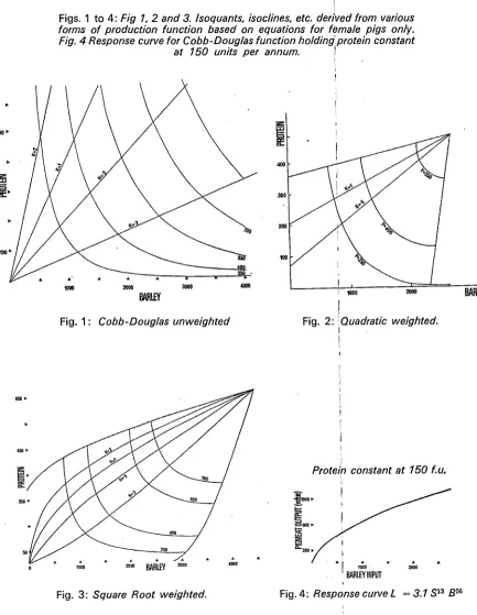
rates o f substitution between them. To expedite the selection process the char acteristics and implications o f each function have been tabulated. In addition, Figs. 1, 2 and 3 present the isoquants and isoclines associated with the equations for females (weighted2 2 in the case o f the quadratic and square root functions.)
From the tabulation it is apparent that, in many ways, the square root function is a compromise between the Cobb-Douglas and Quadratic forms. Many features o f the Cobb-Douglas, such as constant returns to scale and no defined maximum, conflict with such knowledge as exists on production logic, and warrant its rejection as an unsuitable form. Figure 4 shows that the Cobb-Douglas response curve tends to flatten out as input increases, so that, even where (as in this case)23
diminishing returns to scale occur, no maximum is defined. Unless an economic optimum is defined for small magnitudes o f input, the Cobb-Douglas will overestimate the input requirements which equate marginal revenue and marginal
T A B L E 6: Tabulation of main features of selected forms of the production function and their
implications for the respective isoquant maps.
Characteristics etc. Cobb-Douglas Quadratic Square Root
1. Returns to scale (in this specific case)
Constant (sum of exponents
= i - o i -04)
Diminishing and ne gative at high inputs
2. Marginal productivity Declines at declin-of inputs ing rate
Decline at constant rate
Decline at declin ing rate 3(a) Declining total
product
Impossible Yes
3(b) maximum none clearly defined
4. Elasticity of production
constant declines at constant rate
declines at declin ing rate 5. Rate of input
substitution
constant ranges from zero tc infinity 5. Rate of input
substitution
declines at constant rate
declines at declining rate
6. Optimum mix of inputs at different output levels
constant changing proportions
7. Zero inputs yield zero output negative output 8. Production possible
on one input
no yes, on barley alone
9. Low levels of both small positive output negative output below threshold input inputs yield levels
Feature of Maps* GEOMETRIC PRESENTATION
Interval between
isoquants (1.) constant
widening
Ridgelines (3b, 5)
Isoclines (3 a, 6, 7, 8)
Isoquants at low levels of output (9)
same as axes linear converging on maxium linear fan out from linear converging
origin on m a x i m u m asymptotic to axes cut axes
curvilinear con verging on origin and maximum curvilinear con
verging on origin and maximum tend to be asymptotic but may cut axes near origin
t
Figs. 1 to 4: Fig 1, 2 and 3. Isoquants, isoclines, etc. derived from various
forms of production function based on equations for female pigs only. Fig. 4 Response curve for Cobb-Douglas function holding protein constant
at 150 units per annum. I
BARLEY
Fig. 1 : Cobb-Douglas unweighted Fig. 2: Quadratic weighted.
[image:14.490.32.465.67.626.2]j
Fig. 3: Square Root weighted. Fig. 4: Response curve L = 3.1 S1 3 B5 (
i
t
t
cost. Modifications which would make the Cobb-Douglas more flexible, make i t also difficult to compute.
The possibility o f output based on one input is a strong point in favour o f the quadratic and square root functions. However, Australian research24 found that,
while pigs performed exceptionally well on skim alone, they failed to fatten on a diet exclusively o f wheat—the reverse o f what is implied by the Danish work, p The concept 'of a threshold quantity, necessary for maintenance, after which the
pigs grow, is also reasonable.
Fig. 5: Scatter diagram showing Annual Output Response (lb. dwt.)
from 150 f.u. of Protein and variable amounts of Barley.
500 * „
£3
s
treatment average fifth treatment
,200 1400 1600 1800 »<W
F.U. BARLEY
Both the quadratic and square root functions defined maxima which lay far beyond the range o f observations.25 This meant that before a choice could be made
between these functions a more fundamental question needed answering: did the data cover the relevant range o f inputs? Scatter diagrams, such as Figure 5, were plotted to relate barley intake to pigmeat output at given protein levels. These showed that, at lower levels o f energy, the ability o f the pigs to consume was fairly constant, though the ability to convert barley to pigmeat varied considerably. Thus, at the 150 protein level, energy intake at barley level 2 ranged from 1,221 to 1,256 units, while output varied from 323 to 391 lb. In this case the " p i g " consuming 1,221 units produced the 391 lb. o f output. A t level 4 of barley, the range in intake was greater, i.e., 1,637 to 1,745 while the variation in output was less, i.e., 374 to 434. A t the highest level of barley (level 5), the 24. G. E . Battese, L . H . Duloy, J. M . Holder, and B. R. Wilson, "The determination of optimal rations for pigs fed milk and grain", Journal of Agricultural Economics, Vol. X E X , No. 3, 1968.
ability to consume was even more varied, 1,713 to 1,938; and output was again
dispersed, 395 to 452. t Now it is a Well known phenomenon in studies o f animal nutrition that the
"component on genetic variability increases with increases in the level of feeding plane".2 6 On examination, the variances o f treatments were found to vary con
siderably. A t the two lower levels of protein, there was no1 significant difference
in the levels o f intake or output at the two highest levels o f barley feeding. A t the highest level o f protein, there were significant differences but the difference in output was less significant than that for intake. Clearly, the pig's appetite, and its capacity to convert food to meat, were becoming even more significant elements with increasing intensity o f feeding. Protein was' a limitational factor at higher levels o f barley; but increases in protein tended to emphasise the dis parity in the performance o f the individual pigs. This aspect o f the experiment seemed to imply that very little would be gained by extending the levels o f treatment in the way economists often suggest. The presencejof heteroscedasticity, or unequal variances, would vitiate the results of fitting the equations to the data. To overcome this, a weighted regression was fitted, using as weights the inverse of the within treatment variances in the dependent variable. Since, for a given barley treatment, the actual amount of energy received can vary between animals, the above estimates o f error variance may be biased upwards because part o f the within treatment variation is caused by differences in the level o f energy received by the animals on a particular treatment. However, the amount o f bias involved seems reasonably small (roughly about 10 per cent, or less,j of within treatment
T A B L E 7: Regression Coefficients and related statistics for selected forms of production functions
based on weighted data i
Equation Values Independent Variable
Goodness of fit (T)
Constant Term Name w Value of Coefficient S.E. of Coefficient • LINEAR both sexes
•9339 -12-63 s •37569 •01599
(•9316) B •21521 •00792
males
•9372 -33-38 S •34786 •02401
(•9350) B •22762 •00781
females
•8939 8-494 S •42270 •026895
(•8902) B •18703 •01100
I V: Value Level of Significance3 23-50 27-16 14-49 29-13 1572 17-01 * * * * * * * * **** **»* • # * * * * # * *
26. R . T . Plank and A . Berg, "The heritance and plane of nutrition in Swine. 1, Effect of season plane of nutrition, sex and sire on feed lot performance and carcase characteristics", Canadian
E C O N O M I C S P E C I F I C A T I O N O F T H E N E O C L A S S I C A L P R O D U C T I O N F U N C T I O N 239
T A B L E 7—continued
Equation Valu ?s Independent Variable
Goodness Constant Name Value of S.E. of Level of
of fa W Term w Coefficient Coefficient Y Value Significance3 QUADRATIC CROSS PRODUCT
both sexes
•9550 —200-96 s •867294 •117040 7-41 ****
(•953o) •409115 •082666 4-95 #***
s2 —-001117 •000190 5-87 ****
B — -000078 •000028 2-81 *** SB •000096 •000059 1-64 *
males
•9718 -235-40 S •600495 •150559 3-99 ****
(•9692) •489223 •081805 5-98 ****
s* — -000649 •000254 2-56 ** B — -000096 •000027 3-52 #*#* SB •000073 •000059 1-23
females
•9574 -196-30 S ,1.02539 •147456 695 ****
(•9534)
\
•393022 •102425 3-84 ****S — •001438 •000219 6-57 • ^ ^ 'f-B — -000086 •000034 2-55 *** SB •000138 •000077 1-78 *
SQUARE ROOT
both
•9553 -807-37 S -•871563 •218924 3-98 ****
(•9533) B — •230916 •158464 1-46
S 32-2703 77707 4-15 ##** B 29-5870 12-5322 2-36 **#*
SB •22362 •14425 1-55 **
males
•9717 - 8 9 4 7 6 s • -•356201 •295204 I-21
(•9691) B -•317652 •158644 2-00 ***
S 17-5068 10-1512 1-72 ***# B 39-2182 12-7126 3-08 **** SB •139382 •142163 0-98
females
•9559 — 854-10 S 1-20424 •250431 4-81 ****
(-9518) B -•290338 •192979 1-50
S 40-2370 9-59303 4-19 #*** B 30-2445 15-5239 1-95 **** SB •330880 •192844 1-72 **
(1) First value relates to R2, second value i.e. within brackets relates to adjusted R2. (2) S means Soya bean meal and other protein rich feed;
B means barley; both measured in fodder units.
i
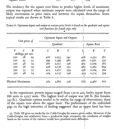
[image:18.488.48.445.199.645.2]variation), as indicated by the scatter diagrams plotted. The results27, given in
Table 7 are based on separate weighting factors calculated for males and females
separately and combined. | The choice between the quadratic and square root form was made in the light
o f the weighted equations (which are those used to plot Figures 2 and 3). The maximum levels o f physical output were, in lb. annually: j
Males Females ; Both
Quadratic 634 576 j 622 Square Root 817 677 804
The tendency for the square root form to predict higher' levels o f maximum output was repeated when optimum outputs were calculated over the range o f likely movements in price ratios and between the inputs themselves. Some typical results are shown in Table 8. [
j
T A B L E 8: Optimum inputs and output at various price levels is based on the quadratic and square
root functions for female pigs only j
Optimum Inputs and Outputs I
Unit prices of ' •—-j
Quadratic i
I Square Root
Y 5 B S B Y 1 B Y
shillings per cwt. J
250 28 24 416 2,055 543 456 2,332 58i 250 33 33 399 1.5.99 480 420 1,921 530 250 48 24 387 2,031 536 403 2,279 567 300 28 24 428 2,156 553 482 2,565 604
300 33 33 413 i , 9 7 i 534 448 2,164 562
300 48 24 404 2,137 548 434 I
2,514 594
Physical Maximum 482 2,667 576 670 4,467 677
In the experiment, protein inputs ranged from 150 to 42Q, barley inputs from 888 units to 2,037 units. The highest level o f output was '568 lb. (for females, 543 lb.). Quadratic optima tended to be within the range o f observations; those o f the square root above the upper limit. The performance o f the individual pigs on the high intensities of feeding suggested that an upper limit has been
reached, and that the quadratic, with its lower maximum levels, reflected better the underlying realities.
Isoquant and Isocline Analysis
A n interesting sidelight on the selection process is obtained by juxtaposing Figures 2, 3 and 4 and examining the map in the area o f economic interest, i.e., between the 250 and 550 lb. isoquants, and between the isoclines appropriate when the unit price o f protein is the same as, and when it is twice, that o f barley, i.e., k = i'0, and k = 0-5. The 250 isoquants are very similar and the
inter-Fig. 6: Superimposition of selected isoquants and isoclines from Figs. 1, 2
and 3.
1000 2000 3000 4000
BAftilY
242 E C O N O M I C A N D S O C I A L R E V I E W !.
i
Regression based on group averages |
Geary2 8 has shown that, where residuals are regular, grouping of observations
leads to very little loss o f efficiency in the estimates. In this study the residues were not regular. Nevertheless it seemed worthwhile to' experiment with a regression based on the 15 group averages. These averages .would replace the scatter o f observations at the higher levels o f input by an estimation o f central tendencies for each treatment. In particular, it would emphasise the flatness of the
upper end o f the regression line. j
T A B L E 9: Regression Coefficients and related statistics for the Quadratic Cross Product form
of function based on treatment averages '
Equation Values Independent Variable
Goodness Constant Name Value of S.E. of 1 Level of (3) of fit (1) Term (*) Coefficient Coefficient Y| Value Significance
Both Sexes i t
•9953 -239-5568 S •79905 •14503 t 5-5i ****
(•9922) B •477H •08882 j 5-37 ****
S2 — -00099 •00018 5-49 **** B2 — -oooio •00003 1 3-86 ****
SB •00010 •00006
j
1-69
Males i
•9946 -305-3164 S •62414 •16682 ! 374 ****
(•9910) B •58270 •09871 ] 5'90 #*#*
S2 — -00052 •00021 • 2-49 * * B2 — -00012 •00003 ' 4-23 ****
SB •00001 •00007 1 0-18
Females 1
•98999 -163-1838 S •94533 •20650 ,4-58 ***
(•9832) B -36250 •12929 2-80 ***
S2 — -00143 •00025 J5-63 **** B2 — -00008 •00004 ] 2-05 *
SB •00020 •00008 J2-3I I
****
N.B. The other forms of
\
equation were also fitted to the treatment average data. (1) First value relates to R2, second value i.e. within brackets relates tojadjusted R2. (2) S means Soya bean meal and other protein rich feed; j
B means barley; both measured in fodder units. j
(3) **** significant at o-i%; * * * a t i % ; **at5%; * a t i o % .
T h e parameters obtained, a n d presented i n T a b l e 9, w e r e used to predict b o t h the physical m a x i m a a n d the o p t i m a u n d e r one set o f prices ( f r o m T a b l e 7, i.e., 250, 28 a n d 24) a n d the results c o m p a r e d w i t h those d e r i v e d f r o m the equations based o n the w e i g h t e d i n d i v i d u a l observations.
T A B L E 10: Comparison of predictions derived from equations based on treatment averages and
those based on weighted individual observations.
Max.
Treatment Averages
Optimum Max.
Weighted Individuals Optimum
Y Y S JJ Y Y S B
Males 592 566 513 2,013 633 601 503 2,248 Females 599 561 438 2,147 576 543 4 i 6 2,055 B o t h Sexes 586 577 45i 2,063 622 586 436 2,270
T h e w e i g h t e d regressions predict higher output a n d higher barley input than do the treatment average equations relating to males a n d b o t h sexes. A l l w e i g h t e d equations indicate l o w e r protein inputs. C o m p a r e d w i t h the group average equations, the w e i g h t e d equations displayed a considerable difference i n the m a x i m u m a n d o p t i m u m output o f males vis-a-vis females. Nevertheless, b e i n g based o n all the data, the w e i g h t e d regression estimates w e r e preferred. T h e striking feature o f the group average regressions w a s the similarity o f their predictions to those o f the w e i g h t e d equations. I n this they w e r e clearly superior as predictive tools to the u n w e i g h t e d equations.
Selection of Variables
H a v i n g selected an equation f o r m , the question r e m a i n s — h o w to treat variables w h o s e coefficients are not significant at, say, the 10 per cent level ( B2 i n t w o instances a n d SB i n the case o f males only) 2 T h e r e is n o sure answer to this, since research w o r k e r s m a y quite rationally differ i n the w e i g h t they attach to logical a n d statistical criteria. S o m e prefer to start out w i t h an initial hypothesis about the appropriate algebraic f o r m o f the equation, a n d tend to retain all coefficients, e v e n i f their standard errors are relatively large. T o t h e m , the predictive p o w e r o f the entire equation is m o r e important than the interpretation o f the i n d i v i d u a l regression coefficients. O t h e r s w i l l o n l y retain those coefficients w h i c h are signi ficant at the conventional 5 per cent probability level.
t I.
244 E C O N O M I C A N D S O C I A L R E V I E W j
I
positive reaction between barley and protein, which it implies, was found to be appropriate when the data was subjected to an analysis of variance at the outset of the study. It should be noted that the fitting of quadratic equations commonly results in only the linear term having significant coefficients.!
Backfat Thickness as an Index of Quality 1
So far the discussion has assumed that one lb. of pigmeat output is as good as another; and the recommended procedure has been in general to feed high levels of both protein and barley. This assumption can now be relaxed and cognisance taken of the influence of feeding on quality. As this was a Danish experiment, the thickness of backfat was presented as a measure of quality, j
Average backfat thickness is not an adequate measure of grade under Irish conditions, so the relationship between it and Irish grading needs to be established. Irish regulations use four grading criteria'—length and backfat thickness at shoulder, midback and loin. A report by Lucas, McDonald' and Calder2 9 stated that a reduction in the level of feeding was unlikely to affect length, but would probably result in reductions in shoulder and backfat thickness, up to a maximum of 10 and 6 mm. respectively.
If length is unaffected by feeding plane, the problem reduces to finding the probability that pigs of a particular backfat thickness will b'elong to a specified Irish grade based on three fat measurements. This was estimated by studying the grade distribution of 1,082 Irish pigs for which backfat measurements were available.30 For example, the study reported 128 pigs with backfat thickness in the interval 30-8 to 31-8 mm. O f these, 31 were "A special", 96 "A" and 1 "B".
Application of the appropriate grade prices would give the weighted average price to be expected for this thickness interval. Since the experimental results recorded the backfat thickness of each pig, all the information was now available to calculate the value of output. There is, however, one difficulty. Not only does the absolute level of the pigmeat price fluctuate but the margins between grades widen and narrow almost continuously31 The problems this introduces are discussed elsewhere.32 This paper uses the weighted average of weekly quotations published by major bacon curers in the period July, 1968 j to June, 1969. In, shillings per cwt. deadweight these were: 2 8 9 , 2 8 0 , 2 5 9 , 249 and 242 for the grades of A special, A, B i and C respectively. |
The two equation approach j
The first approach to introducing quality consideration was to attempt to define [
29. I.A.M. Lucas, I. McDonald and A.S.C. Calder, "Some further observations upon the effects of varying the plane of feeding for pigs between weaning and becon weight", Journal of
Agricultural Science, Vol. 54, p. 81 et seq. j 30. M . Ross, unpublished study, 1965. j 31. See M.Ross, Economics of Pig Production, Economic Research Series No. 6, An Foras Taluntais.
Dublin, 1962. 1
unit prices of output, Py, as a function of protein and barley. This was done in
two stages
P „ = / ( F ) and F = / ( S, B )
i.e., backfat thickness (F) is a function of the inputs, and unit price (Py) is a function
of backfat thickness.
Using the above prices for the range 29*3 to 45*3 mm. in the backfat scale gave:-—•
Py = 385-26 - 3-087 F mm. (A)
Starting at 285/- per cwt. for pigmeat with a backfat of 29-3 mm., each additional mm. of fat would reduce the price by 3 / - a cwt.
The next step was to relate backfat (F) to level of inputs. The most acceptable forms tested were:—
F = 23-8 - - 0 0 5 8 s + -oo86B R2-393 (-386) (B) [•0030] [-00112]
which shows that protein reduces fat, and therefore improves grade, while barley has the opposite effect. The coefficient of S was significant at the 6-0 per cent level; that for B was significant at o-i per cent. The value of R2 is low; but for 120 observations is significant at the o-i per cent level. If protein is not regarded as having a favourable influence on fat formation, then equation B could be formulated in terms of barley only.
F mm. = 21-3 + -0092 B R2 -377 (-372) (C)
F mm. = 27-6 - j - -00000317.B2 R2 '3^2 (-377) (D) [•00000037]
B and JB2 were significant at the o-i per cent level.
Substituting equation B in equation A gives:
p
y = 311-8 + -0179s - -0265s. (E)The use of protein raises the unit price while feeding barley lowers it, through
their respective influences on fat formation. ;
Optimising the Product of Two Functions
The next step is to find the optimising strategy. Given as before that profit is the margin between revenue and cost, i.e.
where TT is profit and the summation sign represents all other costs which are more or less held constant, their optimising conditions are:'—
bS ybS bS 1
I
bT~ lyb~B + ^"oB -Pb = o j
Where Py is a constant (i.e., grading is not considered) the middle term disappears,
and we are left with the partial derivatives of Y equal to the inverse of the prices. When Py is itself a function of 5 and B , the equations become more complex. Substitution of the values for Y and Py, and collecting the terms, results in a pair
of simultaneous quadratic equations in 5 and B . j
266-83 - -6655 + -oi4B - -oooo6S2 - -000004B2 + -oooo6SB = Ps (F) 132-98 + -014s — -070.8 + -00003s2 — -ooooo6B2 — -oo'ooo8SB = P& (G)
Given the values of Pb and Ps, these equations can be solved by an iterative
process. j
The alternative iterative process assumption—price unrelated to protein
An analysis of variation indicated that there was a significant positive relation ship between the level of protein consumption and backfat. This relationship was not strongly confirmed by equation B above, where the coefficient of S was only significant at the 6 per cent level.3 3 If protein is not regarded as influencing backfat, equation E must be recalculated to incorporate equation C : —
Py = 319*52. — -02845 j E(a)
which in turn would yield two further quadratic equations F (a) and G (a) for solution by the iterative procedure. j
The above presentation assumes a linear relationship between price and backfat.
A regression based on 1962 prices34 took the form:— i
Py=— 652-7 + 82-8F - 2-45F2 + - 0 2 F3 + -000003F4.
If equation B was substituted for F in each term the technical difficulties in obtaining an optimum would prove insoluble. [
33. In the co-ordinated trials in Britain, which covered many different locations, breeds of pigs, housing and management conditions but a uniform feeding regime protein, the level of protein was not found to be related to quality, but the experiment was somewhat different, see R. Braude,' M . Townsend, G . Harrington and J. G . Rowell, "Effects of different protein contents in the rations of growing fattening pigs", Journal of Agricultural Science, 55, 2, i960.
The Quasi-Production Function Approach
An alternative approach to incorporating quality would be to value output at the unit price appropriate to its associated backfat, and to calculate a new set of regressions with "value of output" as the dependent variable, in preference to "volume of output". Since quality is inversely related to the level of barley fed, the lower unit prices of higher outputs would have the effect of dampening down
T A B L E I I : Some derived data relating to various equations forms fitted to data giving
in input physical terms and output in monetary terms [prices used for optimising were
Ps=28, Pb=22)
Sex
Maximum Output* Optimum Output Optimum Inputs Coefficients of TiptpTtmn/itinvt T Sex
Financial Physical V V
Financial Physical Protein Barley
-"^ X*'Clt,liiiliwuvri j
1 v— • V V
Q U A D R A T I C F O R M S
group averages
Both 1,260 559 1,225 52o 442 1,773 •9860 (-9789)
Male 1,145 522 1,125 486 382 1,786 •9724 (-9571)
Female 1,266 557 1,228 512 418 1,771 •9833 (1-9740)
Unweighted individual observations
Both 1,312 639 1,266 556 440 1,922 •8309 (-8234)
Male 1,298 796 1,258 553 508 1,837 •8487 (-8347)
Female 1,310 624 1,263 539 421 1,883 •8626 (-8499)
Weighted individual observations
Both 1,316 586 1,270 541 466 1,899 •8925 (-8878)
Male 1,234 547 1,210 506 370 i,735 •9258 (-9189)
Female 1,280 543 1,244 509 440 1,767 •9294 (-9229)
S Q U A R E R O O T F O R M S
group averages
Both 1,329 610 1,263 537 523 1,815 •9877 (-9809)
Female i , i 5 3 540 1,133 497 458 1,588 •9756 (^620)
Male 1,334 622 1,260 530 462 i,854 •984O (-9751)
Unweighted Individual Observations
Male 1,481 696 1,363 591 812 1,796 •8518 (-8381)
Female 1,397 748 1,300 564 470 1,984 •8637 ( - 8 5 I I )
Weighted individual observations
Both 1,440 656 1,337 567 579 2,002 •8935 (-8888)
Male i , 3 7 i 632 1,287 549 295 2,159 •9294 (-9229)
Female 1,360 588 1,286 526 504 1,852 •9300 (-9235)
* Obtained by inserting the S and B values derived from the quasi production function into the corresponding physical production function.
!
the upper levels of the response curve. It might also increajse the variance. The degree of "flattening" would be most marked when price differentials between
grades are widest. { All the equation forms examined in defining the production function proper
were fitted once again to this quasi-production function—quasi in the sense that output was not in physical, (Y), but in monetary, (Py. Y), terms. It would be tedious
to give all the details for each equation fitted. Instead, some 'derived information about each form is presented in Table x i . The linear and Cobb-Douglas forms are omitted since neither produced meaningful optima. I:
T A B L E 12: Comparison of optima obtained output is paid for om a graded or ungraded
basis 1
f
Without Quality Payments With Quality Payments
Pv=25o Pv=3oo
<
Y S B Y S B \ Y S B
Both 586 436 2,270 597 449 2,380 536 464 1,867
Males 601 503 2,248 611 522 2,330 503 373 1,716 Females 543 416 2,055 553 428 2,156 506 438 1,744
The introduction of quality acts as a correction for unequal variance, since both are greatest at the higher levels of barley intake. Thus, the optima obtained using weighted and unweighted monetary data are not as disparatejas was the case with the physical output. On the contrary, the percentage difference is so small, less than 4 per cent in the most extreme case, as to be insignificant. It is difficult to compare the results from the quasi function with the results obtained where price is not influenced by grade, since it is not clear which average price would provide a fair comparison with the built-in prices in the quasi production function. For that reason, the optimum was based on average prices of both 250 and 300 shillings per cwt. In all cases the weighted forms of the equations have been used. The main result of introducing grade is to cut back barley j feeding. The more conservative reduction, where Py = 250, ranged, nonetheless, from 15 to 25
per cent and was due to the negative correlation between barley inputs and quality. Protein, which tends to be positively correlated with quality, increased, or in the case of males fell, by an amount similar to that of barley.
The greater simplicity of the quasi product approach to introducing quality means that it might be preferred even if it meant new calculations every time the margin between the various grades altered. In practice, sensitivity analysis might reveal that the optimum would not be seriously altered over a considerable range of variations in the price relationship between the individual grades.
The consequence of the alternative approaches to quality 1
protein and barley of 28 and 24 shillings per cwt. were assumed, with the following results:
T A B L E 13: Comparison of optima obtained under various assumptions about quality (calculated
for both sexes only)
1. No quality payments, fixed output price 250/-2. No quality payments, fixed output price 300/-3. Quality payments—quasi production function 4. Two equation approach: protein improves quality35 5. Protein does not improve
s B Y
436 2,270 586 449 2,380 597 464 1,867 536 443 1,965 550 424 1,924 542
The optimal strategy of the "two equation" approach called for less protein, more barley, and higher output than the quasi production function. On the other hand, their optimal barley levels were far below those recommended where grading was not commercially practised. It is for the analyst to decide whether the differences in the last three methods are significant in relation to other uncertainties in the production and sales processes.
In the discussion to date we have attempted to meet the conditions laid down above for selecting a production function which would be an error free guide to decision-making—all inputs to be included, the observations to cover the relevant rangq and the parameters to be specified without error. The form we have selected, if correctly specified, is nonetheless a statistical, rather than a logical function. This means that, strictly speaking, it only applies to the population to which it refers.
The purpose of specifying a function is to provide a guide to producers. Correct specification is half the battle. There still remain the problems of predicting prices and yields. The short lifespan of pigs, and the system of guaranteed prices, mean that reasonably accurate estimates of the general price level can be made. Predicting intergrade margins, while less easy, may still be adequate for manage ment purposes.
Greater uncertainty will normally apply to predictions of yield. Conditions facing producers can never be exactly duplicated in experiments, so there is always some error in transferring experimental data to commercial situations.36
35. An interesting academic sidelight on the results is that given a constant unit price of output the marginal rate of substitution between barley and protein at the optimum which would be 0-786 for a price relationship of 28:22 (i.e. 22-^-28) was, in fact, 0-436 when price was influenced by the inputs of protein and barley.