Experiments on Morphological Reinflection: CoNLL 2017 Shared Task

Experiments on Morphological Reinflection: CoNLL-2017 Shared Task

Akhilesh Sudhakar BITS, Pilani, India

[email protected]

Anil Kumar Singh IIT (BHU), Varanasi, India

[email protected]

Abstract

We present two systems for the task of morphological inflection, i.e., finding a target morphological form, given a lemma and a set of target tags. Both are trained on datasets of three sizes: low, medium and high. The first uses a simple Long Short-Term Memory (LSTM) for low-sized dataset, while it uses an LSTM-based encoder-decoder LSTM-based model for the medium and high sized datasets. The second uses a simple Gated Recurrent Unit (GRU) for low-sized data, while it uses a combination of simple LSTMs, sim-ple GRUs, stacked GRUs and encoder-decoder models, depending on the lan-guage, for medium-sized data. Though the systems are not very complex, they give accuracies above baseline accuracies on high-sized datasets, around baseline accuracies for medium-sized datasets but mostly accuracies lower than baseline for low-sized datasets.

1 Introduction

The CoNLL-SIGMOPRHON 2017 shared task Cotterell et al. (2017) consists of two subtasks out of which we participate only in the first subtask, which involves generating a target inflected form from a given lemma with its part-of-speech. For instance, the word writ-ing is the present continuous inflected form of the lemma write. The models were trained on three differently-sized datasets. The low-sized datasets had around 100 training samples, the medium-sized datasets had around 1000 training samples and the high-sized datasets had around 10000 samples for most languages. Datasets were provided for a total of 52 languages.

2 Background

Prior to neural network based approaches to mor-phological reinflection, most systems used a 3-step approach to solve the problem: 1) String alignment between the lemma and the target (mor-phologically transformed form), 2) Rule extrac-tion from spans of the aligned strings and 3) Rule application to previously unseen lemmas to transform them. Durrett and DeNero (2013) and

Ahlberg et al. (2014;2015) used the above ap-proaches, with each of them using different string alignment algorithms and different models to ex-tract rules from these alignment tables. However, in these kinds of systems, the types of rules to be generated must be specified, which should also be engineered to take into account language-specific transformational behaviour.

Faruqui et al.(2016) proposed a neural network based system which abstracts away the above steps by modeling the problem as one of generating a character sequence, character-by-character. Akin to machine translation systems, this system uses an encoder-decoder LSTM model as proposed by

Hochreiter and Schmidhuber(1997). The encoder is a bidirectional LSTM, while the decoder LSTM feeds into a softmax layer for every character po-sition in the target string. A beam search is used to create many output sequences and the best one is chosen based on predicted scores from the soft-max layer. This model takes into account the fact that the target and the root word are similar, ex-cept for the parts that have been changed due to inflection, by feeding the root word directly to the decoder as well. A separate neural net is trained for every language.

3 System Description

We have modeled our system based on the system proposed by Faruqui et al. (2016), as described

in the previous section. However we have made some modifications to the above system, to ac-count for the three different sizes of datasets and to account for the behaviour of morphological trans-formations of independent languages. We submit-ted two submissions for the shared task, each of which we describe in the following sections.

In all the models, some structural and hyper-parametrical features remain the same. The acters in the root word are represented using char-acter indices, while the morphological features of the target word are represented using binary vec-tors. Each character of the root word is then em-bedded as a character embedding of dimension 64, to form the root word embedding. If an encoder is used, it is bidirectional and the the input word em-beddings feed into it. The output of the encoder (if any), concatenated with the root word embed-ding, feeds into the decoder. All recurrent units have hidden layer dimensions of 256, meaning that they transform the input to a vector of dimension 256. Over the decoder layer is a softmax layer that is used to predict the character that must oc-cur at each character position of the target word. In order to maintain a constant word length, we use paddings of ’0’ characters. All models use cate-gorical cross-entropy as the loss function and the Adam optimizer as reported by Kingma and Ba

(2014) for optimization.

3.1 First Submission

3.1.1 Low-sized Dataset

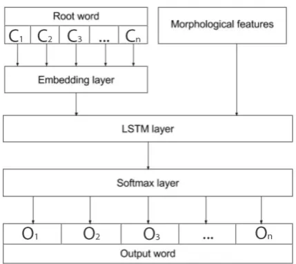
For training the model on the low-sized dataset, we did not use any encoder and we used a sim-ple LSTM with a single layer as the recurrent unit (Figure 1).

3.1.2 Medium-sized Dataset

For training the model on the medium-sized dataset, we used a bidirectional LSTM as the en-coder and a simple LSTM with a single layer as the decoder (Figure 2).

3.1.3 High-sized Dataset

For training the model on the high-sized dataset, we used a bidirectional LSTM as the encoder and a simple LSTM with a single layer as the decoder (Figure 2).

Figure 1: C1, .., Cn represent characters of the

root word whileO1, .., Onrepresent characters of

the output word

3.2 Second Submission 3.2.1 Low-sized Dataset

For training the model on the low-sized dataset, we did not use any encoder and we used a sim-ple GRU, as reported byCho et al. (2014), with a single layer as the recurrent unit (Figure 3).

3.2.2 Medium-sized Dataset

For medium-sized dataset, we used different model configurations for different languages. Four different kinds of configurations were used:

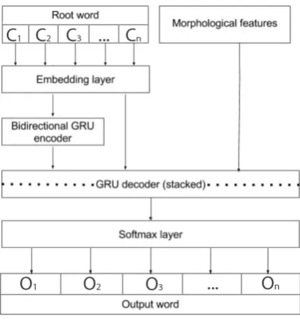
1) Bidirectional LSTM as the encoder and a simple LSTM with a single layer as the decoder (Figure 2) 2) Bidirectional GRU as the encoder and a simple GRU with a single layer as the de-coder (Figure 4) 3) No ende-coder and a simple GRU with a single layer as the recurrent unit (Figure 3) 4) Bidirectional GRU as the encoder and a deep GRU (two GRUs stacked one above the other) as the decoder (Figure 5)

The specific configuration used for each lan-guage has been listed in Table 1. The configura-tion numbers indicated in the table are according to those mentioned above.

3.2.3 High-sized Dataset

Configuration Language List

1 Arabic, Basque, Bengali, Catalan, Georgian, Latin, Quechua, Urdu

2 Kurmanji

3 Bulgarian, Czech, Estonian, Faroese, German, Icelandic, Irish, Latvian, Lithuanian, Norwegian-Bokmal, Persian, Polish, Swedish

4 Albanian, Armenian, Danish, Dutch, English, Finnish, French, Haida, Hebrew, Hindi, Hungarian, Italian, Khaling, Lower-Sorbian, Macedonian, Navajo, Northern-Sami, Norwegian-Nynorsk, Portuguese, Romanian, Russian, Scottish-Gaelic, Serbo-Croatian,

Slovak, Slovene, Sorani, Spanish, Turkish, Ukrainian, Welsh

Table 1: Configurations for different languages for medium-sized data for submission-2.

Language B S-1(T) S-2(T) Norwegian-Bokmal 69.0 52.6 62.7 Danish 59.8 46.1 49.8

Urdu 30.3 31.2 43.7

Hindi 31.0 33.4 40.8

Swedish 54.3 40.6 39.4

Table 2: Accuracies for top-5 languages for low data.

Language BL S-1 S-2 Quechua 68.1 93.0 93.0 Bengali 75.0 91.0 91.0 Portuguese 92.9 86.0 89.6 Urdu 86.1 88.0 88.0 Georgian 90.0 87.7 87.7

Table 3: Accuracies for top-5 languages for medium data.

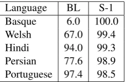
Language BL S-1 Basque 6.0 100.0 Welsh 67.0 99.4 Hindi 94.0 99.3 Persian 77.6 98.9 Portuguese 97.4 98.5

Table 4: Accuracies for top-5 languages for high data.

Language BL S-1 S-2

Norwegian-Bokmal 0.489 0.71 0.55 Danish 0.669 0.95 0.87 Swedish 0.884 1.08 1.09 Norwegian-Nynorsk 0.928 1.41 1.23

Dutch 0.69 1.42 1.24

Table 5: Levenshtein distances for top-5 languages for low data.

Figure 2: C1, .., Cn represent characters of the

root word whileO1, .., Onrepresent characters of

the output word

some ablation studies on high-size datasets, which have been discussed in the analysis section.

4 Evaluation

4.1 Results on Test Set

Figure 3: C1, .., Cn represent characters of the

root word whileO1, .., Onrepresent characters of

the output word

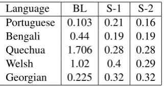
Language BL S-1 S-2 Portuguese 0.103 0.21 0.16 Bengali 0.44 0.19 0.19 Quechua 1.706 0.28 0.28 Welsh 1.02 0.4 0.29 Georgian 0.225 0.32 0.32

Table 6: Levenshtein distances for top-5 languages for medium data.

The complete set of accuracies and Levenshtein distances for all languages have been included in Appendix-1 (tables 8 to 10), sorted by accuracies. The main observation from these tables is that languages belonging to the same language family tend to get similar similar results by our system, which is intuitively valid (although there are many exceptions). For example, Romance and Slavic languages tend to occur together in these tables.

However, it is not evident from these tables that morphologically more complex languages should be harder to learn, which seems to be

counter-Language BL S-1 Basque 3.32 0.0 Serbo-Croatian 0.36 0.0 Welsh 0.45 0.01 Hindi 0.075 0.02 Persian 0.567 0.02

Table 7: Levenshtein distances for top-5 languages for high data.

Figure 4: C1, .., Cn represent characters of the

root word whileO1, .., Onrepresent characters of

the output word

intuitive. For example, Turkish is above French. This may be because of hyperparameters or con-figurations selected for different languages (which were different, in an attempt to maximize accuracy on the development data).

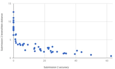
Figures 6 to 10 show the correlation between accuracy and Levenshtein distance for all three sizes of datasets for submission-1 and for low and medium sizes of datasets for submission-2.

4.2 Ablation Studies

While we were unable to run an exhaustive hy-perparameter search due to lack of time, we per-formed some experiments, where the choice of hy-perparameters was guided by intuitions developed from analysis of the dataset and results obtained on smaller subsets of the data. We have presented some key observations from our analysis in the en-suing sub-sections.

4.2.1 Early Stop Patience

Figure 5: C1, .., Cn represent characters of the

root word whileO1, .., Onrepresent characters of

the output word

Figure 6: Accuracy vs. Levenshtein Distance for high data (submission-1)

6-8 while for high-sized datasets, it can be set to around 3-4. However, in order to ensure best re-sults, we set our patience value to 10 across all models, training sizes and languages in the final system.

4.2.2 External Feature Categories

In last year’s version of the shared task, the morphological features in the dataset were annotated along with the category of each feature. For instance, a sam-ple training feature set from last year is: ‘pos=N,def=DEF,case=NOM/ACC/GEN,num=SG’. This year, however, the category of each feature was not provided, i.e., the same example above would appear in this year’s format as:

Figure 7: Accuracy vs. Levenshtein Distance for medium data (submission-1)

Figure 8: Accuracy vs. Levenshtein Distance for low data (submission-1)

’N,DEF,NOM/ACC/GEN,SG’. Our studies show that while it is conceptually true that the presence of feature categories means exploring a shorter search space, the absence of them does not make a difference to the accuracies obtained for high and medium sized datasets. In the case of low-sized datasets, marginally better accuracies (around 0.5-1%) were obtained when the categories were incorporated into the dataset (this was done manually). However, this might also be the effect of random initialization of parameters.

Figure 10: Accuracy vs. Levenshtein Distance for low data (submission-2)

4.2.3 Choice of Recurrent Unit

Simple Recurrent Neural Networks (RNNs) per-formed the poorest on all sizes of datasets. For low-sized datasets, in almost all cases, using a GRU gave better results than using an LSTM. On an average, the accuracy increased by 2.33% when shifting from LSTM to GRU as the choice of re-current unit.

In the case of medium-sized datasets, 8 out of 52 languages performed better with an LSTM than a GRU, while the rest showed better performance with a GRU.

4.2.4 Convolutional Layers

We also ran experiments using convolutional lay-ers, in which the root word was convolved and the convolution was concatenated along with the root word and passed to the encoder layer (if any). The rest of the network structure remained the same. For low-sized and medium-sized datasets, adding convolutional layers resulted in the accuracy drop-ping to near 0. For high-sized datasets, we were unable to finish running the experiments on all lan-guages due to lack of time. However for the few languages on which we performed convolutional ablation studies, it did seem to improve accuracy by around 1.5% on an average.

4.2.5 Stacking Recurrent Units

Deeper models (more than one layer of LSTM/GRU) resulted in drastic accuracy drops for low-sized datasets. For medium-sized datasets, 30 out of 52 languages showed an accuracy improvement upon stacking two GRU layers, while the accuracy drop in the rest 22 was not drastic but appreciable.

5 Conclusions

There are two main conclusions. One is that differ-ent configurations of deep neural networks work well for different languages. The second is that deep learning may not be the right approach for low-sized data.

Results for low-size were poor for almost all languages. It is to be noted that we used purely deep learning. If deep learning is augmented with other transduction, rule-based or knowledge-based methods, the results for low-size could perhaps be improved.

For high-sized data, for one language (Basque), we even got an accuracy of 100%. For medium, the highest was 93% and for low, the highest was 69%.

References

Malin Ahlberg, Markus Forsberg, and Mans Hulden. 2014. Semi-supervised learning of morphological paradigms and lexicons. InProc. of the 14th Con-ference of the European Chapter of the Association for Computational Linguistics:Language Technol-ogy (Computational Linguistics). Gothenburg, Swe-den, pages 569–578.

Malin Ahlberg, Markus Forsberg, and Mans Hulden. 2015. Paradigm classification in supervised learning of morphology. InProc. of the 2015 Conference of the North American Chapter of the Association for Computational Linguistics: Human Language Tech-nologies. Denver, Colorado, pages 1024–1029. Kyunghyun Cho, Bart van Merrienboer, Caglar

Gul-cehre, Fethi Bougares, Holger Schwenk, and Yoshua Bengio. 2014. Learning phrase representations using rnn encoder-decoder for statistical machine translation. InProc. of EMNLP 2014.

Ryan Cotterell, Christo Kirov, John Walther G´eraldine Sylak-Glassman, Ekaterina Vylomova, Patrick Xia, Manaal Faruqui, Sandra K¨ubler, David Yarowsky, Jason Eisner, and Mans Hulden. 2017. The conll-sigmorphon 2016 shared task: Universal morpho-logical reinflection in 52 languages. InProc. of the CoNLL-SIGMORPHON 2017 Shared Task: Univer-sal Morphological Reinflection. Vancouver, Canada. Greg Durrett and John DeNero. 2013. Supervised learning of complete morphological paradigms. In Proc. of the 2013 Conference of the North American Chapter of the Association for Computational Lin-guistics: Human Language Technologies. Atlanta, Georgia, pages 1185–1195.

Sepp Hochreiter and J¨urgen Schmidhuber. 1997. Long short-term memory. Neural Comput. 9(8):1735– 1780.

Diederik P. Kingma and Jimmy Ba. 2014. Adam: A method for stochastic optimization. CoRR abs/1412.6980.

Acknowledgement

We would like to thank Shaili Jain, Aanchal Chaurasia and Himanshu Karu for their help in our experiments in this shared task.

Appendix-1

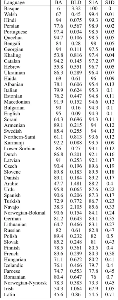
In Tables 8 to 10 (on this page and the next), BA stands for baseline accuracy, BLD for baseline Levenshtein Distance, S1A for submission-1 ac-curacy, S1LD for submission-1 Levenshtein Dis-tance, S2A for submission-2 accuracy and S2LD for submission-2 Levenshtein Distance. All three tables are sorted by submission-1 accuracy, since we have results for all dataset sizes for this sub-mission.

Language BA BLD S1A S1D

Basque 6 3.32 100 0

Welsh 67 0.45 99.4 0.01

Hindi 94 0.075 99.3 0.02

Persian 77.6 0.567 98.9 0.02

Portuguese 97.4 0.034 98.5 0.03

Quechua 94.7 0.106 98.5 0.05

Bengali 84 0.28 98 0.05

Georgian 94 0.111 97.5 0.04

Khaling 53.8 0.816 97.4 0.04

Catalan 94.2 0.145 97.2 0.07

Hebrew 55.8 0.551 96.7 0.05

Ukrainian 86.3 0.289 96.4 0.07

Haida 69 0.61 96 0.09

Albanian 78.1 0.606 95.4 0.13

Italian 79.9 0.624 95.3 0.1

Estonian 76.2 0.447 94.8 0.11

Macedonian 91.9 0.152 94.6 0.12

Bulgarian 90 0.16 94.3 0.1

English 95 0.09 94.3 0.1

Sorani 64.3 0.696 94.3 0.11

Armenian 89.1 0.215 94 0.12

Swedish 85.4 0.255 94 0.13

Northern-Sami 61.1 0.813 93.6 0.12

Kurmanji 92.2 0.088 93.5 0.09

Lower-Sorbian 86 0.27 93.1 0.12

Dutch 86.8 0.201 92.1 0.16

Latvian 91 0.253 92.1 0.17

Czech 90.4 0.196 89.6 0.19

Slovene 89.8 0.183 89.5 0.18

Danish 89.1 0.184 89.2 0.17

Arabic 47.7 1.481 88.2 0.4

Urdu 95.8 0.065 87.6 0.22

Spanish 90.6 0.206 87.3 0.17

Turkish 72.9 0.772 86.7 0.23

Navajo 38.3 2.105 85.6 0.33

Norwegian-Bokmal 90.6 0.154 84.1 0.24

German 81.2 0.643 83.1 0.35

Lithuanian 64.7 0.466 83.1 0.27

Russian 82 0.61 82.8 0.47

Polish 89.4 0.232 82 0.5

Slovak 85.2 0.248 81 0.43

Finnish 78.5 0.361 80.5 0.4

French 83.6 0.299 80.3 0.38

Hungarian 71.1 0.622 80.2 0.41

Icelandic 76.1 0.466 79.7 0.4

Faroese 74.7 0.553 77.8 0.45

Romanian 80.4 0.647 76 0.7

Norwegian-Nynorsk 78.3 0.383 73.3 0.45

Irish 54.3 1.064 67.9 1.05

Latin 45.6 0.86 54.5 0.71

Language BA BLD S1A S1D S2A S2D

Quechua 68.1 1.706 93 0.28 93 0.28

Bengali 75 0.44 91 0.19 91 0.19

Urdu 86.1 0.287 88 0.47 88 0.47

English 90.2 0.159 87.9 0.2 0 8.74

Georgian 90 0.225 87.7 0.32 87.7 0.32

Portuguese 92.9 0.103 86 0.21 89.6 0.16

Hindi 86.6 0.186 85.2 0.56 87.4 0.42

Haida 56 1.24 83 0.47 0 17.48

Kurmanji 88.4 0.234 81.6 0.62 19.2 1.72 Catalan 83.2 0.337 79.7 0.38 79.7 0.38

Turkish 33.1 2.854 74.5 0.65 0 12.97

Welsh 54 1.02 74 0.4 83 0.29

Macedonian 82.3 0.323 69.3 0.5 79.1 0.32

Danish 78.1 0.336 69.2 0.47 0.5 5.53

Spanish 85.4 0.322 66.7 0.89 73.9 0.68

Dutch 71.7 0.403 66.5 0.62 74.6 0.44

Basque 2 5.11 66 0.75 66 0.75

Scottish- 52 0.76 66 1.04 76 0.68

Gaelic

French 76.1 0.45 63.6 0.77 69.7 0.61

Italian 73.8 0.743 58.5 1.26 70.3 0.8

Armenian 76.6 0.442 58.4 1.14 68.1 0.78 Latvian 85.1 0.278 57.7 0.95 60.2 0.88

Persian 65.4 1.068 57.1 1.27 57 1.46

Hebrew 40 0.933 55.9 0.69 65.8 0.51

Bulgarian 75 0.445 54.8 1.13 55.5 0.98

Slovak 70.7 0.533 52.8 0.82 63.7 0.6

Khaling 18.4 1.909 52.2 0.97 58.2 0.81 Norwegian- 79.8 0.311 48.7 0.74 78.3 0.33

Bokmal

Hungarian 41.7 1.559 47.7 1.05 62.8 0.68

Swedish 73.7 0.452 47.7 1 70 0.49

Sorani 52.8 1.053 46.5 1.31 57.5 0.95

Estonian 62.4 0.779 39.9 1.68 45.7 1.63

Russian 75 0.737 39.4 1.37 66.6 0.83

Serbo-Croatian 65.8 0.884 38.7 1.83 49.5 1.52

Czech 80.7 0.434 38.6 1.74 52.9 1.41

Arabic 40 1.787 37.6 2.2 37.6 2.2

Romanian 70.2 0.848 36.9 1.95 49 1.57

Northern-Sami 35.7 1.445 34 1.64 40.8 1.26 Lithuanian 53 0.714 33.7 1.34 37.6 1.34

Slovene 81.9 0.33 32.3 1.13 73.5 0.45

Albanian 66.1 1.175 32.2 2.44 41.5 1.88 Ukrainian 71.5 0.538 30.8 1.47 61.5 0.7

German 71.5 0.798 30.1 1.49 57.3 0.93

Latin 36.8 1.103 22.1 1.72 22.1 1.72

Irish 44.7 1.457 20.1 3.71 26.1 3.11

Navajo 31.3 2.495 19.9 2.82 19.3 2.78

Polish 75.2 0.533 19.6 2.01 48.4 1.33

Finnish 42.5 1.353 15 3.21 21.5 2.75

Faroese 58.7 0.891 0 8.13 40.4 1.2

Icelandic 61.4 0.763 0 8.09 41.6 1.16

Lower-Sorbian 70.5 0.587 0 7.01 69 0.52 Norwegian- 63.3 0.634 0 8.68 56.4 0.71

Nynorsk

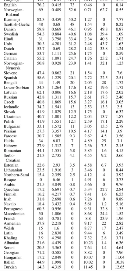
Table 9: Results for all languages for medium data, sorted by submission-1 accuracy

Language BA BLD S1A S1D S2A S2D

English 76.2 0.415 73 0.46 0 8.14

Norwegian- 69 0.489 52.6 0.71 62.7 0.55 Bokmal

Kurmanji 82.3 0.459 50.2 1.27 0 7.77

Scottish-Gaelic 48 0.68 48 1.54 0 8.32

Danish 59.8 0.669 46.1 0.95 49.8 0.87

Swedish 54.3 0.884 40.6 1.08 39.4 1.09

Hindi 31 3.798 33.4 2.34 40.8 2.02

Urdu 30.3 4.201 31.2 2.48 43.7 1.63

Dutch 53.7 0.69 28.2 1.42 33.8 1.24

German 53.7 1.111 25.6 1.75 0 8.59

Catalan 55.2 1.091 24.7 1.76 25.2 1.71

Norwegian- 50.8 0.928 23.9 1.41 32.1 1.23 Nynorsk

Slovene 47.4 0.862 21 1.54 0 7.6

Spanish 58.6 1.229 20.1 2.72 22.5 2.51

Bengali 44 1.49 20 2.05 28 1.72

Lower-Sorbian 34.3 1.264 17.6 1.82 19.6 1.72

Latvian 62.1 0.806 16.6 2.18 17.6 2.02

Russian 42.8 1.311 15.7 2.61 17.3 2.46

Czech 40.8 1.869 15.6 3.27 16.1 3.05

Icelandic 34.2 1.541 13 2.53 13.3 2.5

Slovak 41.9 1.029 12.5 1.75 0 6.32

Ukrainian 40.7 1.001 12.2 2.04 13.7 1.87

Polish 41.9 1.551 12.1 2.59 17.1 2.29

Bulgarian 33.1 1.572 11 3.05 13.5 2.78

Persian 27.3 3.357 10.5 4.17 14.1 3.9

Faroese 30.7 1.585 9.3 2.62 4.5 3.56

Haida 34 6.03 7 4.89 25 3.1

Hebrew 27.9 1.312 7 2.36 7.5 2.15

Romanian 44.1 1.551 5.8 3.85 1.6 4.15

Serbo- 21.3 2.735 4.1 4.55 9.2 3.66

Croatian

Estonian 22.6 2.93 3.5 4.58 6.7 3.93

Lithuanian 23.5 1.916 3 3.46 0 8.44

Northern-Sami 15.4 2.359 2.5 4.12 4 3.92

Basque 0 6.46 1 4.91 6 3.73

Arabic 21.5 3.049 0.8 5.66 0 9.76

Quechua 17.2 6.691 0.7 5.34 22.7 2.84

Finnish 16.2 4.217 0.7 7.41 1.6 6.53

Irish 31.8 2.698 0.6 7.26 0 9.89

Navajo 18.4 3.432 0.4 5.61 1.2 5.16

Portuguese 60.3 0.956 0 9.31 32.8 1.35

Macedonian 50 1.006 0 8.68 24.4 1.52

French 63 0.781 0 8.8 23.9 1.96

Armenian 37.8 2.218 0 9.17 22 2.82

Welsh 15 1.6 0 8.77 17 2.47

Latin 16 2.838 0 9.44 6 3.49

Khaling 3.9 4.298 0 7.32 2.8 3.71

Albanian 21.6 4.439 0 10.23 1.4 6.36

Sorani 20.5 3.363 0 7.64 1.4 4.64

Georgian 71.2 0.585 0 8.82 0 7.96

Hungarian 17.2 2.049 0 10.07 0 11.04

Italian 44.9 1.998 0 10.02 0 10.38

Turkish 14.3 4.319 0 11.45 0 12.65