Abstract— A fixed-structure controller based on robust H loop shaping control is proposed in this paper. It can be used to guarantee the robust performance under a structure-specified controller. In this proposed technique, Particle Swarm Optimization (PSO) is applied in the design controller, and the inverse of infinity norm from disturbances to states is formulated as the objective function in searching the optimal controller. Simulation results of MIMO electro-hydraulic servo system show that the proposed controller has simpler structure than that of the conventional Η∞ loop shaping controller and its
stability margin is near the Η∞ loop shaping controllers.
Index Terms— fixed-structure robust H loop shaping, Particle Swarm Optimization, MIMO electro-hydraulic servo system
I. INTRODUCTION
he Electro-hydraulic servo systems are well known. Electro-hydraulic actuator is an attractive choice for being used in both industrial and non-industrial applications because of the following fast dynamic response, high power to inertia ratio and control accuracy. Controlling of these systems is important because of their highly nonlinear. In recent years, the robust control has received much attention that can be guarantee for system under conditions of uncertainty, parameter changes, and disturbances. However, the robust controllers are difficulty in practical applications. The simple controller such as PI, PID controller is today’s most commonly used control in servo systems. This problem extends the gap between the theoretical and practical approaches.
To solve this problem, the design of a fixed-structure robust controller has been proposed and has become an interesting area of research because of its simple structure and practicable controller order. In [1], a robust H∞ optimal
control problem with a structure specified controller was solved by using genetic algorithm (GA). As concluded in [1], GA is a simple and capable method to design a fixed-structure H∞ optimal controller. B.S. Chen. et. al. [2]
proposed a PID design algorithm for mixed H2/H∞ control.
In their paper, PID control parameters were tuned in the stability domain to achieve mixed H2/ H∞ optimal control. A
This work was supported in part by Faculty of Engineering, King Mongkut’s Institute of Technology Ladkrabang, Bangkok, Thailand.
Piyapong and Somyot are with the Department of Electrical Engineering, Faculty of Engineering, King Mongkut’s Institute of Technology Ladkrabang, Bangkok 10520, Thailand. Email : [email protected].
similar idea was proposed in [3] by using the intelligent GA to solve the mixed H2/H∞ optimal control problem.
However, the fixed structure controller based on H∞ optimal
control designed in [1-3] are difficulty for both the uncertainty of the model and the performance are essentially chosen weights.
Alternatively, a fixed structure H∞ loop shaping
controller is proposed by [4-5]. A. Umut Genc in 2000 [4] adopted the concept of state space approach and BMI optimization. As shown in this research, specifying the initial solution has a huge effect on the optimal solution because of the local minima problem. S. Patra et.al. in [5] designs an output feedback robust controller that has the same structure as the pre-compensator weight which is normally designed by PI. Though the fixed structure H∞
loop shaping control techniques mentioned above are easy to select weighting function, they requires only two specified weights, pre- and post-compensator weights [6], for shaping the nominal plant so that the desired open loop shape is achieved. Fortunately, the selection of such weights is based on the concept of classical loop shaping, which is a well known technique in controller design.
However, the resulting controller in [4-5] is always ineffective and the problem of local minima often occurs in the design. To solve these problems, searching algorithms such as genetic algorithm, particle swarm optimization technique, tabu-search, etc., can be employed. In this paper, we proposed a new design technique by the PSO based fixed-structure robust H∞ loop shaping control. PSO is
employed to find the parameters of the controllers. The structure of controller in the proposed technique is selectable; in this paper, the fixed-structure robust PI controller is designed. Simulation results show that a controller designed by the proposed approach has a good performance and robustness as well as a simple structure.
The remainder of this paper is organized as follows. Section II covers the MIMO Electro-hydraulic Servo system modeling. In section III, conventional Η loop shaping and the proposed technique are discussed as well as PSO algorithm. The design examples and results are demonstrated in section IV. And in section V the paper is summarized.
II. MODELING
MIMO electro-hydraulic servo system is shown in Fig. 1 which consists of a position control system and a force control system [7]. The position control system which is used to control the actuator movement and the force control system which is used to supply a required force to the
Structure Specified Robust
H
Loop Shaping
Control of a MIMO Electro-hydraulic Servo
System using Particle Swarm Optimization
Piyapong Olranthichachat and Somyot Kaitwanidvilai
system load. The objective of the electro-hydraulic servo system is to satisfy the requirements such as zero steady state errors in motion of the actuator and force output.
Force Transducer
Servo value Controller Force Actuator
Servo value
Controller Position Actuator
Position sensor
Force Control System
Position Control System
F2 y1 u2 u1 Position Input Force Input + +
-Fig.1. MIMO electro-hydraulic servo system
The state-space of the MIMO electro-hydraulic servo system is
x Ax Bu y Cx
(1)
The dynamic model of this system is an MIMO system which has 2 outputs (y), F2 – force of the system and y1 –
position of the actuator, and 2 inputs (u), u1 – input servo
value of the position control system, and u2 – input servo
value of the force control system.
III. CONVENTIONAL HLOOP SHAPING CONTROL AND
PROPOSED TECHNIQUE
A. Conventional Η∞ Loop Shaping Control
Η∞ loop shaping control [6] is an efficient method to
design a robust controller. This approach requires only a desired open loop shape in frequency domain which is specified by the weighting functions, pre-compensator (W1)
and post-compensator (W2). The uncertainty model of the
system is formulated as normalized co-prime factors that divide the shaped plant (Gs) into nominator factor(Ns) and
denominator factor (Ms) which is shown in Fig.2.
Consequently, the shaped plant can be written as:
1 2
s
G W GW (2)
1
( )( )
s s Ns s Ms
G N M (3) where ∆Ns and ∆Ms are the uncertainty transfer functions
in the nominator and denominator factors, respectively.
∆Ns, ∆Ms∞ , where is the stability margin. The
determination of the normalized co-prime and the solving of the Η∞loop shaping control can be seen from [8].
∆Ns ∆Ms
Ns Ms-1
+ -+ + K -Gs
Fig.2. Co-prime factor robust stabilization problem.
In this approach, the pre-compensator (W1) and
post-compensator (W2) weights for achieving the desired loop
shape are defined then optimal stability margin (opt) is
solved by the following equation.
1 ( ) 1 1
inf
opt opt s s
stab K
I
I G K M
K
(4)
If the (opt) is too low, then go to select new weighting
function. Select the stability margin (<opt) and then
synthesize the controller, K∞, by solving the following
inequality.
1 1 1 1 ( ) ( )zw s s
s s
I
T I G K M
K
I
I G K I G
K
(5)The feedback controller (K) is
1 2
K W K W (6)
B. Proposed Technique
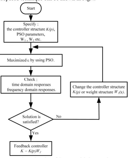
The proposed technique begin with determining the structure of the controller (K(p)). The parameter, p, of the controller is changeable. Then, PSO is used to find the right parameter, p. In robust problem, the stability margin () is single index to indicate performance of the designed controller which is obtained as follows.
11 ( )1
zw s s
I
T I G K I G
K (7)
Where K∞ can be found by KW K p W11 ( ) 21. Suppose
that W1 andW2 can be inversed. Generally, W2 is chosen to
be equal to identity matrix I. Therefore, objective function can be written in this form:
1 1 1 1 1 1 1 ( ( )) ( ) zw s sObjective function T
I
I G W K p I G
W K p
(8)
For this design of controller, the controller K(p) will be designed to minimize the infinity norm from disturbance to state (Tzw ) or maximize ( ) by PSO method. This method
is capable in solving many engineering problems. Fig. 3 shows the swarm’s movement which is the basic idea of PSO. As seen in this figure, a bird represents the particle and the position of each particle represents the candidate solution. Moreover, it is requires only upper, lower bounds of solution and PSO parameters such as the population of swam(n), lower and higher boundary (pmin , pmax) of the
problem, minimum and maximum velocity of particles (vmin
, vmax), minimum and maximum iteration(imax). PSO is an
iterative algorithm. In each iteration, the value of fitness (fs) of each population in the ith generation is calculated. Then,
choose the population that gives the highest fitness value to use as the answer of the generation. The inertia weight (Q), value of velocity (v) and position (p) of each population in the present generation (i) are updated by using this equation (9), (10) and (11), respectively.
max min
max
max
Q Q
Q Q i
i
1 1[ (1 )] 2[ 2( )]
i i i b i i b i
v Qv P p U p (10)
1 1
i i i
p
p
v
(11)Where 1 , 2 are acceleration coefficients
[image:3.595.53.292.108.274.2]1i , 2i are any random number in (0→1) range
Fig. 3. The movement of a swarm.
Based on the PSO technique, in this problem, sets of controller parameters p is formulated as a particle and the fitness can be written as:
1
1 1
1 1
1
( ( ) )
( )
0.0001
s s
I
I G W K p I G
Objective function W K p
[image:3.595.314.541.166.434.2]…(12) From (13); fitness value will be defined to equal a constant with very little value. The controller from particle makes the system unsteady. The flow chart of the design of the proposed technique can be shown in Fig.4.
Fig. 4. Flow chart of the proposed design procedure.
IV. SIMULATION RESULTS
The state-space of a nominal plant can be seen in [7]. The state vector of this plant consists of the four variables which
are supply pressure in force control system, supply pressure in position control system, position of the actuator and velocity of the actuator. The details of this plant are given in appendix A. In this paper, the pre- and post-compensator weights are chosen as:
1 2
0.8 60
0 1 0
0.001 ,
0.8 60 0 1
0
0.001
s s
W W
s s
(13)
In this paper, the structure of controller is selected as:
1 2 3 4
5 6 7 8
0.001 0.001 ( )
0.001 0.001
p s p p s p
s s
K p
p s p p s p
s s
(14)
100 101 102 103 104 -50
-40 -30 -20 -10 0 10 20 30 40 50
Singular Values
Frequency (rad/sec)
S
ing
ul
ar
V
al
ues
(
dB
)
Fig.5. Singular values (--plant), ( Shaped plant) of MIMO electro-hydraulic servo system.
Singular values of MIMO electro-hydraulic servo system and desired loop shape are plotted in Fig.5. As seen in this figure, the bandwidth and performance are significantly improved by the compensator weights. The shaped plant has large gains at low frequencies for performance and small gains at high frequencies for noise attenuation. With these weighting functions, the robust requirement is satisfied.
By using (13), the optimal stability margin of the shaped plant is found to be 0.7034. This value indicates that the selected weights are compatible with robust stability requirement in the problem. To design the conventional Η∞
loop shaping controller, stability margin 0.6682 is selected. As a result, the final controller (full order Η∞loop shaping
controller) is 8th order and complicated.
In the optimization problem, the upper and lower bounds of control parameters and PSO parameters are given in Table 1.
Table 1 PSO parameters and controller parameters range.
Parameter value minimum velocities 0
[image:3.595.50.276.450.728.2]minimum inertia weights
0.6
maximum inertia weights
0.9
maximum iteration 60 population size 500
p1-8 [-60, 60]
After running the PSO for 60 iterations when running PSO for 33 iterations, the optimal solution is obtained as:
0.5355 34.503 0.1304 2.5367
0.001 0.001
( )
0.0258 2.897 0.3682 36.641
0.001 0.001
s s
s s
K p
s s
s s
(15)
Fig.6 shows the fitness or stability margin ( ) of the controller in each generation. The best answer evolved by PSO has a stability margin of 0.4780.
0 10 20 30 40 50 60
0.2 0.25 0.3 0.35 0.4 0.45 0.5
iterations
S
ta
bi
lity
M
ar
gi
n (
)
Fig.6. Stability margin ( ) versus iteration.
0 0.05 0.1 0.15 0.2 0.25 0.3 0.35 0.4
0 0.2 0.4 0.6 0.8 1 1.2 1.4
Time (sec)
P
os
iti
on
O
utp
ut
(c
m
)
H loop shaping Proposed Controller
(a)
0 0.05 0.1 0.15 0.2 0.25 0.3 0.35 0.4
-0.02 0 0.02 0.04 0.06 0.08 0.1 0.12
Time (sec)
F
orc
e O
ut
pu
t(k
N
)
H
loop shaping
Proposed Controller
(b)
Fig.7. Output response of the system both when the unit step is entered to position command.
Fig.7 shows the response of the output of the system in 2 channels (input servo value of the position control system and input servo value of the force control system). When the unit step is fed into the position command, it can be found that the proposed controller performs well. Its response is close to the Η∞ loop shaping controller, with no overshoot.
Fig.8 shows the responses of the system when unit step is fed into force command.
0 0.05 0.1 0.15 0.2 0.25 0.3 0.35 0.4
-0.01 0 0.01 0.02 0.03 0.04 0.05 0.06 0.07 0.08 0.09
Time (sec)
P
os
iti
on
O
utp
ut
(c
m
)
H loop shaping Proposed Controller
(a)
0 0.05 0.1 0.15 0.2 0.25 0.3 0.35 0.4
0 0.2 0.4 0.6 0.8 1 1.2 1.4
Time (sec)
F
orc
e O
ut
pu
t(k
N
)
H loop shaping Proposed Controller
(b)
V. CONCLUSION
This paper presents a new technique for designing a fixed structure robust H loop shaping controller which proposed technique can be applied a robust controller for a MIMO electro-hydraulic servo system. In the proposed can select structure of controller. Based on the notion of classical H loop shaping, stability margin () is used to indicate robustness and performance of the proposed controller. This parameter is defined as the objective function of searching the optimal solution by PSO method. In this technique make easy because PSO simplifies the method. Simulation results demonstrate that the proposed technique is adjustable and reasonable.
APPENDIX
In this paper, the linearized model of the MIMO electro-hydraulic servo system is taken from [7], that is
65.58 59.98 18.02 14.15
25.98 121.5 0 25.98
12.45 12.38 84.65 0
0.99 0.91 21.53 61.52
A
17.79 0 158.1 0.13
4.68 79.8
0 0
B
0 1.07 0 0
0 0 1 0
C
0 0 0 0
D
REFERENCES
[1] B. S. Chenand Y. M. Cheng. (1998), A structure-specified optimal control design for practical applications: a genetic approach,” IEEE Trans. on Control System Technology, Vol. 6, No. 6, pp. 707-718.
[2] B. S. Chen, Y.-M. Cheng, and C. H. Lee. (1995), A genetic approach
to mixed H2/ H∞ optimal PID control, IEEE Trans. on Control
Systems, pp.51-60.
[3] S. J. Ho, S. Y. Ho, M. H. Hung, L. S. Shu, and H. L. Huang, Designing structure-specified mixed H2/ H∞ optimal controllers
using an intelligent genetic algorithm IGA (2005), IEEE Trans. on Control Systems, 13(6), pp.1119-24.
[4] A. U. Genc, “A state-space algorithm for designing Η loop shaping
PID controllers,” technical report., Cambridge University, Cambridge, UK, Oct. 2000.
[5] S. Patra, S. Sen and G. Ray. (2008) Design of static Η∞ loop shaping
controller in four-block framework using LMI approach. Automatica, 44, pp. 2214-2220.
[6] McFarlane, D., Glover, K. (1992). A loop shaping design procedure using Η∞ synthesis. IEEE Transactions on Automatic Control, 37(6), pp. 759-769.
[7] Hao Zhang, Neural adaptive control of nonlinear MIMO eletrohydraulic servo system, Spring, 1997.
[8] S. Skogestad & I. Postlethwaite, Multivariable Feedback Control Analysis and Design. 2nd ed. New York: John Wiley & Son, 1996.
[9] J. Kennedy and R. Eberhart, Particle swarm optimization, IEEE