Abstract—Good rosters have many benefits for an organization, such as lower costs, more effective utilization of resources and fairer workloads and distribution of shifts. The process of constructing optimized work timetables for the personnel is an extremely demanding task, hence the use of decision support systems for workforce scheduling has become increasingly important for both the public sector and private companies. This paper describes an effective method for optimizing large-scale staff rostering instances. The idea is to divide an instance into smaller units, solve them separately and then combine the results together again. A set of artificial and real-world instances derived from the actual instances solved for various companies are presented. We publish the best solutions we have found using our computational intelligence heuristic called the PEAST algorithm. We invite the workforce scheduling community to challenge our results. This research has contributed to better systems for our industry partner.
Index Terms—Staff Rostering, Large-Scale Real-World Scheduling, Workforce Scheduling, Computational Intelligence.
I. INTRODUCTION
Workforce scheduling, also called staff scheduling and labor scheduling, is a difficult and time consuming problem that every company or institution that has employees working on shifts or on irregular working days must solve. The workforce scheduling problem has a fairly broad definition. Most of the studies focus on assigning employees to shifts, determining working days and rest days or constructing flexible shifts and their starting times. Different variations of the problem are NP-hard and NP-complete [1]-[8], and thus extremely hard to solve. The first mathematical formulation of the problem based on a generalized set covering model was proposed by Dantzig [9]. Good overviews of workforce scheduling are published by Alfares [10], Ernst et al. [11] and Meisels and Schaerf [12].
Nurse rostering [13] is by far the most studied application area in workforce scheduling. Other successful application areas include airline crews [14], call centers [15], check-in counters [16], ground crews [17], nursing homes, call centers and airport ground services [18], postal services
N. Kyngäs is with the Satakunta University of Applied Sciences, Pori, Finland (phone: +358 50 542 9219; fax: +358 2 620 3030; e-mail: [email protected]).
J. Kyngäs is with the Satakunta University of Applied Sciences, Pori, Finland (e-mail: [email protected]).
K. Nurmi is with the Satakunta University of Applied Sciences, Pori, Finland (e-mail: [email protected]).
[19], transport companies [20] and retail stores [21]. Recent successful algorithms for staff scheduling include ant colony optimization [22], dynamic programming [23], constraint programming [24], genetic algorithms [25], scatter search [26], hyperheuristics [27], integer programming [28], metaheuristics [29], simulated annealing [30], tabu search [31] and variable neighborhood search [32].
The need for effective commercial workforce scheduling has been driven by the growth of the customer contact center industry and retail sector, in which efficient deployment of labor is of crucial importance. The balance between offering a superior service and reducing costs to generate revenues must constantly be found.
There are five basic reasons for the increased interest in workforce scheduling optimization. First, public institutions and private companies around the world have become more aware of the possibilities of decision support technologies, and they no longer want to handle the schedules manually. Second, human resources are one of the most critical and most expensive resources for these organizations. Careful planning can lead to significant improvements in productivity. Third, good schedules are very important for the welfare of the staff. They also reduce sick-leaves. Besides increasing employee satisfaction, effective labor scheduling can also improve customer satisfaction. Fourth, new algorithms have been developed to tackle previously intractable problem instances, and, at the same time, computer power has increased to such a level that researchers are able to solve real-world problems. Finally, one further significant benefit of automating the scheduling process is the considerable amount of time saved by the administrative staff involved.
The goal of this paper is to describe an effective method for solving large-scale staff rostering instances as they occur in various lines of business and industry. Section II introduces the workforce scheduling process and necessary terminology. Section III gives an outline of our computational intelligence algorithm. In Section IV we describe how to divide a staff rostering instance into smaller units, solve them separately and then combine the results together again. Section V presents a set of artificial test instances and Section VI a real-world instance. We publish the best solutions we have found and invite the workforce scheduling community to challenge our results.
We believe this is the first publication that uses a computational intelligence heuristic to divide and combine large-scale staff rostering instances, and furthermore, present artificial and real-world benchmark instances. We hope these instances will lay the foundation for the standard
Optimizing Large-Scale Staff Rostering
Instances
benchmark instances for the problem. II. WORKFORCE SCHEDULING
Workforce scheduling consists of assigning employees to tasks and shifts over a period of time according to a given timetable. The planning horizon is the time interval over
which the employees have to be scheduled. Each employee has a total working time that he/she has to work during the planning horizon. Furthermore, each employee has
competences (qualifications and skills) that enable him/her
to carry out certain tasks. Days are divided into working days (days-on) and rest days (days-off). Each day is divided
into periods or timeslots. A timeslot is the smallest unit of
time and the length of a timeslot determines the granularity of the schedule. A shift is a contiguous set of working hours
and is defined by a day and a starting period on that day along with a shift length (the number of occupied timeslots).
Shifts are usually grouped in shift types, such as morning,
day and night shifts. Each shift is composed of a number of
tasks. A shift or a task may require the employee assigned to
it to possess one or more competences. A work schedule for an employee over the planning horizon is called a roster. A
roster is a combination of shifts and days-off assignments that covers a fixed period of time.
Table I shows a solution for a simple one-week workforce scheduling instance with seven employees, two shifts (day and night) in a working day and one of three tasks to be completed within a shift. Moreover, tasks A and B cannot be carried out by Bea and Ellie, a night shift cannot be followed by a day shift on the next day, and each employee should have exactly one day-off.
TABLEI
AN EXAMPLE OF A WORKFORCE SCHEDULING SOLUTION
Axel Bea Cass Dave Ellie Fay Gary
Mon Day Night C B A A C B
Tue Day A B C
Night C A B
Wed Day Night C A B A C B
Thu Day Night C B A A B C
Fri Day B A C
Night A C B
Sat Day Night C C A B B A
Sun Day A C B
Night B C A
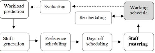
We classify the real-world workforce scheduling process as given in Fig. 1. Workload prediction, also referred to as
demand forecasting or demand modeling, is the process of determining the staffing levels - that is, how many employees are needed for each timeslot in the planning horizon. In this presentation, workload prediction also includes determination of planning horizons, competence structures, regulatory requirements and other constraints.
Shift generation is the process of determining the shift
structure, tasks to be carried out on particular shifts and the competence needed on different shifts. The shifts generated
[image:2.595.306.556.155.240.2]from a solution to the shift generation problem form the input for subsequent phases in the workforce scheduling. Another important goal for shift generation is to determine the size of the workforce required to solve the demand. Shifts are created anonymously, so there is no direct link to the employee that will be eventually assigned to the shift.
Fig. 1. The real-work workforce scheduling process.
In preference scheduling, each employee gives a list of
preferences and attempts are made to fulfill them as well as possible. The employees’ preferences are often considered in the days-off scheduling and staff rostering phases.
Days-off scheduling deals with the assignment of rest days
between working days over a given planning horizon. Days-off scheduling also includes the assignment of vacations and special days, such as union steward duties and training sessions. Staff rostering, also referred to as shift scheduling,
deals with the assignment of employees to shifts. It can also specify the starting time and duration of shifts for a given day, even though in most cases they are preassigned in shift design. In other words, days-off scheduling deals with working days and staff rostering deals with the working times of day. When days-off and shifts are scheduled simultaneously, the process is sometimes called tour
scheduling. Another special case is to schedule days-off
every tenth week and roster staff every second week to enable the employees to plan their free time more conveniently.
The phases from shift generation to staff rostering can be solved using computational intelligence. Computational workforce scheduling is a key to increased productivity, quality of services, customer satisfaction and employee satisfaction. Other advantages include reduced planning time, reduced payroll expenses and ensured regulatory compliance.
Rescheduling deals with ad hoc changes that are
necessary due to sick leaves or other no-shows. The changes are usually carried out manually. Finally, participation in
evaluation ranges from the individual employee through
personnel managers to executives. A reporting tool should provide performance measures in such a way that the personnel managers can easily evaluate both the realized staffing levels and the employee satisfaction. When necessary, the workload prediction and/or shift generation can be reprocessed and focused, and the whole workforce scheduling process restarted.
III. THE COMPUTATIONAL INTELLIGENCE ALGORITHM
generated solutions and the algorithmic power of the algorithm (i.e. its efficiency and effectiveness). Other important criteria include flexibility, extensibility and learning capabilities. We can steadily note that our PEAST algorithm [35] realizes these criteria. It has been used to solve world school timetabling problems [36], real-world sports scheduling problems [37] and real-real-world workforce scheduling problems [38].
The PEAST algorithm is a population-based local search method. As we know, the main difficulty for a local search is
1) to explore promising areas in the search space - that is, to zoom in to find local optimum solutions to a sufficient extent, while at the same time,
2) avoiding staying stuck in these areas for too long and 3) escaping from these local optima in a systematic
way.
[image:3.595.47.294.405.666.2]Population-based methods use a population of solutions in each iteration. The outcome of each iteration is also a population of solutions. Population-based methods are a good way to escape from local optima. Our algorithm is somewhat based on the cooperative local search method [39]. In a cooperative local search scheme, each individual carries out its own local search, in our case the GHCM heuristic [40]. The outline of the algorithm is given in Fig. 2. and the pseudo-code of the algorithm is given in Fig. 3
Fig. 2. The population-based PEAST algorithm.
The reproduction phase of the algorithm is, to a certain extent, based on steady-state reproduction: the new schedule replaces the old one if it has a better or equal objective function value. Furthermore, the least fit is replaced with the best one when n better schedules have been found, where n is the size of the population. Marriage selection [41] is used to select a schedule from the population of schedules for a single GHCM operation. In the marriage selection we
randomly pick a schedule, S, and then we try at most k – 1
times to randomly pick a better one. We choose the first better chromosome, or if none is found, we choose S.
Fig. 3. The pseudo-code of the PEAST algorithm.
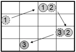
[image:3.595.313.438.653.739.2]The heart of the GHCM heuristic is based on similar ideas to the Lin-Kernighan procedures [42] and ejection chains [43]. The basic hill-climbing step is extended to generate a sequence of moves in one step, leading from one solution candidate to another. The GHCM heuristic moves an object, o1, from its old position, p1, to a new position, p2, and then moves another object, o2, from position p2 to a new position, p3, and so on, ending up with a sequence of moves. Picture the positions as cells as shown in Fig. 4. The initial cell selection is random. The cell that receives an object is selected by considering all the possible cells and selecting the one that causes the least increase in the objective function when only considering the relocation cost.
Fig. 4. A sequence of moves in the GHCM heuristic
Then, another object from that cell is selected by considering all the objects in that cell and picking the one
Set the time limit t, no_change limit m and the population size n Generate a random initial population of schedules
Set no_change = 0 and better_found = 0 WHILE elapsed-time < t
REPEAT n times
Select a schedule S by using a marriage selection with k = 3 (explore promising areas in the search space)
Apply GHCM to S to get a new schedule S’
Calculate the change Δ in objective function value
IF Δ < = 0 THEN Replace S with S’ IF Δ < 0 THEN
better_found = better_found + 1 no_change = 0
END IF ELSE
no_change = no_change + 1 END IF
END REPEAT
IF better_found > n THEN
Replace the worst schedule with the best schedule Set better_found = 0
END IF
IF no_change > m THEN
(escape from the local optimum)
Apply shuffling operators Set no_change = 0 END IF
(avoid staying stuck in the promising search areas too long) Update simulated annealing and tabu search framework Update the dynamic weights of the hard constraints (AdaGen) END WHILE
for which the removal causes the biggest decrease in the objective function when only considering the removal cost. Next, a new cell for that object is selected, and so on. The sequence of moves stops if the last move causes an increase in the objective function value and if the value is larger than that of the previous non-improving move. Then, a new sequence of moves is started. The initial solution is randomly generated.
In our solution to staff rostering in large instances, the PEAST algorithm is used to divide first the employees and then the jobs into groups – that is, to create a partition of the set of all employees/jobs in a certain way. Using the notation above, the employee/job groups are the cells and the employees/jobs are the objects in their corresponding division problems.
The tabu list and simulated annealing refinement [40] are used to avoid staying stuck in the promising search areas for too long. The simulated annealing refinement uses a standard exponential annealing scheme. The annealing is stopped at some predefined temperature. After a certain number of iterations, m, we let the algorithm accept an
increase in the cost function with some constant probability,
p. We choose m equal to the maximum number of iterations
with no improvement to the cost function and p equal to
0.0015. This annealing schedule has been proven to produce better solutions compared to the well-known annealing schedules.
A hyperheuristic [45] is a mechanism that chooses a heuristic from a set of simple heuristics, applies it to the current solution, then chooses another heuristic and applies it, and continues this iterative cycle until the termination criterion is satisfied. We use the same idea, but the other way around. We apply shuffling operators to escape from the local optimum. We introduce a number of simple heuristics that are normally used to improve the current solution but, instead, we use them to shuffle the current solution - that is, we allow worse solution candidates to replace better ones in the current population. In solving the large-scale staff rostering instances, the PEAST algorithm uses three shuffling operations:
1) Select k1 random employees/jobs from random groups and move them into other random groups. 2) Select k2 pairs of random employees/jobs from
random groups, and swap each pair.
3) Select a random group. Select at most k3 random employees/jobs from the group, and move them into other groups.
The algorithm runs for a set number of iterations. For the first half of those, one random shuffling operation is run every 5,000th iteration. For the latter half, a random shuffling operator operator is triggered by 5,000 consecutive iterations without improvement to the solution. For the first half k1, k2 and k3 are all 1. For the latter half their values stochastically vary between 5 and 10.
The algorithm uses an adaptive penalty method (ADAGEN) for multi-objective optimization. A traditional penalty method assigns positive weights (penalties) to the soft constraints and sums the violation scores to the hard
constraint values to get a single value to be optimized. The ADAGEN method assigns dynamic weights to the hard constraints based on the weights assigned to the soft constraints [40]. The soft constraints are assigned constant weights according to their significance.
IV. THE DIVIDE-AND-COMBINE APPROACH FOR LARGE-SCALE STAFF ROSTERING INSTANCES
There are hundreds of workforce scheduling solutions commercially available and in widespread use. In that sense, the so-called implementation-oriented workforce scheduling approach is standard practice in industry. However, we believe there is still a gap between academic and commercial solutions. The commercial products may not include the best academic solutions. We have earlier defined [46] the implementation-oriented staff scheduling research as research that raises
1) such modeling issues that have probably precluded academics from getting their research results implemented to commercial advantage, and
2) the collaboration between an academic researcher, a problem owner and an industry software vendor. According to our experience, the best action plan for real-world workforce scheduling research is to cooperate with both a problem owner and a third-party vendor. In addition, an academic should not consider working with user interfaces, financial management links, customer reports, help desks, etc. Instead, one should concentrate on modeling issues and algorithmic power.
However, it should be noted that it is difficult to incorporate the experience and expertise of the personnel managers into a workforce scheduling system. Personnel managers often have extremely valuable knowledge and experience, and a detailed understanding of their specific staffing problem, which will vary from company to company. To formalize this knowledge into a mathematical business model is not an easy task.
Rostering a large number of employees – roughly speaking more than one hundred - is an extremely demanding task. As the number of employees grows beyond this limit, the computation time needed to find acceptable solutions grows drastically – in most cases to unreasonable levels. This is the problem we address in this paper.
The phase of the workforce scheduling process treated in this paper is staff rostering. Companies often have manual processes for determining days-off schedules, and they are extremely reluctant to let go of them. Our divide-and-combine approach for large staff rostering instances consists of four phases:
1. Divide the employees into N groups
(E1, E2, …, EN) that are as homogeneous as possible with regard to the constraints relevant to the instance at hand.
compatibility between each pair, so that scheduling the jobs of Ji to the employees of Ei has as good an expected result as possible.
3. Roster the staff for each of the N individual
groups, scheduling the jobs in group Ji to the employees in group Ei.
4. Combine the N generated subrosters into one
roster. This is a solution to the original large-scale problem.
In phase one the goal is to make the employee groups statistically as similar to each other as possible. Intuitively this is done to maintain the diversity of the whole set of employees within the groups. Other approaches were also considered during the course of the development process but were abandoned due to their potential pitfalls. The group division is solved using our PEAST algorithm. There are no hard constraints in this phase.
There are a myriad of things that might be considered when constructing employee groups. Some, like shift restrictions and competences, are more important than others. We consider the following in descending order of importance:
1) Shift restrictions of the employees. Each group should contain such employees that for each day and for each shift code (for example, M for morning shift) the number of employees who can do a job with a certain code is the same.
2) Competences of the employees. Like 1), but for competences instead of shift restrictions. In actual implementation, competences and shift restrictions are combined into one constraint, since an employee’s actual ability to work on any given day is highly dependent on both.
3) Shift preferences of the employees. Like 1), but handles employees’ preferred shift codes.
4) Size of the groups.
5) Employees with pre-assigned jobs. The goal is to balance the number of such jobs among the groups for each day.
6) Employees with days-off. Like 1), but for days-off codes instead of shift restrictions.
7) The ending times of the last jobs for employees from the previous planning horizon should be evenly distributed among the groups. Since this only concerns one day and usually only a small number of employees, it doesn’t have a high priority.
Restrictions (Jane has a day-off on Thursday, hence she cannot have a morning shift on Friday) and competences (Abdul cannot drive a bus to a military area since he is not a native citizen) are a primary concern, having a weight of three. All the other constraints have weights of one.
Phase two is somewhat similar to phase one. The major difference is that the job groups are mostly dependent on the corresponding employee groups, whereas the employee groups mostly depend on the number of groups. For example, in phase one, each group should have M / N
employees, where M is the total number of employees and N is the number of groups, whereas group Jk should have as many jobs as the employees of group Ek can do. This phase is also solved using our PEAST algorithm. The things we consider in this phase are as follows:
1) For each group and for each day we must have at least as many available employees as we have jobs. Furthermore, the shift restrictions and competences of the employees must be considered, so that a trivially impossible situation can be avoided (for example, if an employee group has five people who can work the morning shift on a given Monday, there can be at most five morning shifts for that day in the corresponding job group). This is the only hard constraint. This is by far the most important constraint when the instance is difficult.
2) As 1), but instead of ensuring a sufficiently small number of jobs for each group try to balance the differences between the available employees and jobs in each group. This is important for easier instances.
3) The sizes of the groups are matched according to their employee group counterparts.
4) For each group and for each day we try to match the total sum of job minutes with the average minutes the corresponding workers are able to do. Constraint 1) is the only hard constraint. Constraint 2), which balances the available employees based on shift restrictions and competences has a weight of three. The group size balance constraint has a weight of two. All the other constraints have weight of one.
Phase three is again solved using our PEAST algorithm as in [34]. In phase four all the rosters are assembled into one. This is a trivial procedure.
Note that the quality of the solution in phases one and two is often not that apparent until phase four is completed. The hard constraint weights are set so that each hard violation in phase two (phase one contains no hard constraints) causes one hard violation in the final schedule. However, it is mostly impossible to be certain that a particular group structure does not guarantee the existence of additional hard constraint violations in phase three.
V. ARTIFICIAL BENCHMARK INSTANCES
Most of the current staff rostering benchmark instances have rather specialized constraints that not all staff rostering algorithms are capable of tackling. Our goal is to make the instances and constraints as simple as possible, so that a wide range of staff rostering algorithms could be used to solve them. Our artificial instances consist of 1,000 employees and 14,000 jobs. The planning horizon is two weeks. There are no days-off, so each employee should end up with one job for each day - that is, 14 jobs in total. Some of the constraints used here are defined in [46] (each such case noted in parentheses). The following constraints are considered:
1) An employee cannot be assigned to more than one shift per day. This is a hard constraint.
2) An evening shift should not be succeeded by a morning shift. One violation for each such occurrence. (O5)
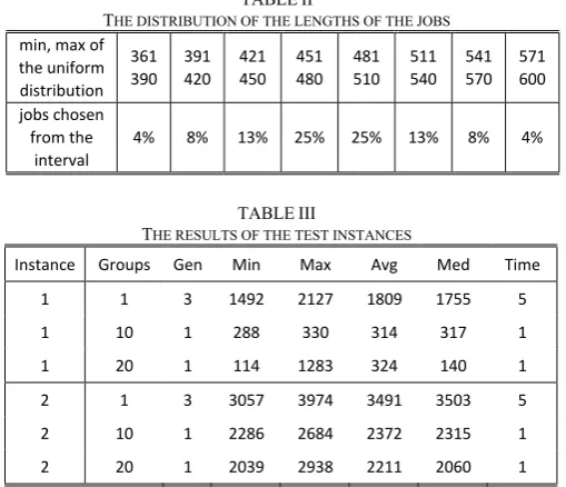
3) The required number of working minutes (6,727 or 6,728 for each employee) should be respected. One violation for each minute of absolute difference between the final and the target value of working minutes for each employee. (R1) Due to the lack of complex constraints, the jobs are essentially different in only three variables: the day of the job, the length of the job and whether it is a morning shift or an evening shift. The instances were generated as follows. For each day we create 1,000 jobs. The lengths of the jobs were chosen as shown in Table II. For example, for each day there are exactly 40 (4% of 1000) jobs between 361 and 390 minutes in length. The exact job lengths were generated using discrete uniform distributions, so on average we choose each job length between 361 and 390 minutes exactly once for each day.
The first instance consists of only morning shifts, so constraint 2) is irrelevant. The second instance was generated from the first one by transforming 50% of the jobs in each day, picked at random, into evening shifts.
Table III shows that the results improve greatly with the group division. This is to be expected. Without the division phase, the running time required by PEAST to achieve acceptable solutions in such a large instance is huge. With group division those solutions are reachable within a reasonable time.
With ten groups, six out of six runs are far superior to the best run made without group division for the first instance. Increasing the number of groups to twenty causes one run out of six to be much worse, while each of the other five runs are better than the best run with ten groups. Thus it seems that the optimal number of groups for this particular instance might be even higher, but it may call for an increase in the number of generations to achieve reliability. In real-world situations the number of generations is usually limited by time constraints, which is an important factor to consider. The metric by which to determine the best set of runs is another important consideration. Using the worst run we would choose ten to be the number of groups for similar data in the future. Using the best run, average run or median run we’d choose twenty groups instead. The number of
generations is smaller for the runs with group division simply to better demonstrate the quality of the solutions and savings in running time provided by the division approach. There were no hard constraint violations in any runs for the first instance. Phase three could be parallelized, which would usually lead to the entire process being faster than simply running PEAST on the whole data with equal number of generations. However, it is simpler to execute simultaneous sequential runs in order to maximize system stability.
TABLEII
THE DISTRIBUTION OF THE LENGTHS OF THE JOBS min, max of
the uniform
distribution
361
390
391
420
421
450
451
480
481
510
511
540
541
570
571
600
jobs chosen
from the
interval
4% 8% 13% 25% 25% 13% 8% 4%
TABLEIII
THE RESULTS OF THE TEST INSTANCES
Instance Groups Gen Min Max Avg Med Time
1 1 3 1492 2127 1809 1755 5
1 10 1 288 330 314 317 1
1 20 1 114 1283 324 140 1
2 1 3 3057 3974 3491 3503 5
2 10 1 2286 2684 2372 2315 1
2 20 1 2039 2938 2211 2060 1
Groups = number of groups the data was divided into, Gen = number of generations (millions) used in the run, Min = the best solution found (in 6 runs), Max = the worst solution found, Avg = the average solution, Med = the median solution, Time = the approximate running time in days. The runs were made on a PC with Intel Core i7-980X Extreme Edition 3.33GHz and 6GB of RAM running Windows 7 Professional Edition.
The results for the second instance are similar to those of the first one. Adding the constraint to reduce morning shifts following evening shifts roughly doubles the value of the objective function for unmodified PEAST. One solution out of six also had one hard constraint violation. The effect of the additional constraint is more pronounced on the dividing approach, yet the results still beat the unmodified version by a fair margin. There were no hard constraint violations in any of the runs made with group division for the second instance. As the number of groups grows from ten to twenty, the variance of the results grows yet again. This time the average solution goes down, though.
VI. AREAL-WORLD BENCHMARK INSTANCE
The real-world instance introduced in this section is based on a case we have solved with our business partner. The detailed data can be obtained from the authors by email.
[image:6.595.302.557.191.410.2]There are a total of 4,522 jobs, and they are 491 minutes in length on average. The job lengths vary between 259 and 648 minutes. The combined length of the jobs is 41,328 minutes below the combined target average shift length of the employees, so, on average, each employee has roughly 76 minutes less work than they should have over the two-week period. The earliest jobs start at 4:35AM and the latest jobs end at 1:28AM. They are split into four categories that are used as preferences for the employees: morning, noon, evening and night.
Again, some of the constraints used here are defined in [46] and in the case of such constraints the name used in [46] are in parentheses. We set out to optimize the following constraints.
1) An employee cannot be assigned to more than one shift per day. This is a hard constraint.
2) A night shift must not precede a day-off. This is a hard constraint. (E8)
3) An employee must have a resting time of 9 hours between two shifts. This is a hard constraint. (R5) 4) The required number of working minutes over the
whole two-week period (459 for each actual working day) must be respected. One violation is given for each minute of absolute difference between the final and the target value of working minutes for each employee. (R1)
5) The shortage of job minutes should be distributed evenly among the employees. Let c be the total of
minute shortage (41,328) divided by the total number of working shifts doable by the employees (4,928). Thus c describes the average
shortage per shift. To get the optimal shortage, s,
for a given employee, c is multiplied by the
number of days-on for that employee. Let d be the
absolute difference between the employee’s shortage and the target shortage. One violation for each minute above 0.1s, rounded up.
6) A night shift should not precede a morning shift or a noon shift. One violation for each such occurrence. (O5)
TABLEIV
THE RESULTS OF THE REAL-WORLD INSTANCES
Groups Gen Min Max Avg Med Time
1 10 5481 7206 6291 6335 5
7 10 312 803 483 462 5
14 10 126 2686 542 256 5
Groups = number of groups the data was divided into, Gen =
number of generations (millions) used in the run, Min = the best solution found (out of ten runs), Max = the worst solution found, Avg = the average solution, Med = the median solution, Time = the
approximate running time in days. The runs were made on a PC with Intel Core i7-980X Extreme Edition 3.33GHz and 6GB of RAM running Windows 7 Professional Edition.
Table IV shows our results for the instance. The runs with group division are far superior to those produced by the unmodified PEAST. Doubling the number of groups from seven to fourteen greatly increases the variance of the runs,
increasing the average slightly yet improving the best run and the median by a notable amount.
The running time may look impractical for real-world applications. However, according to our runs halving the number of generations has surprisingly little effect on the results. In addition to reducing the number of generations, the total running time can be cut to a fraction by parallelizing phase three. This does not mean that the computation time becomes negligible. Based on our experiences, we estimate that almost as good and reliable results (within 10%) as above could be reached with the approximate running time of one day. Considering the fact that the planning horizon is two weeks, that should be more than acceptable. The actual personnel who use the software may need more reinforcement. They may have heard about software that rosters the staff very quickly (maybe within 15 minutes). However, these software solve only distances with a few dozen employees and our software solves instances with hundreds of employees. We find it advantageous to use more computation time in order to achieve better results. It should also be noted that integer programming based optimizers do not usually gain substantial improvement in solution quality when the computation time is increased from e.g. 15 minutes to one day.
VII. CONCLUSIONS AND FUTURE WORK
We described an effective method for optimizing large-scale staff rostering instances. A set of artificial and real-world instances were solved using our computational intelligence heuristic called the PEAST algorithm. This research has contributed to better systems for our industry partner. Our future research will include staff demand forecasting and shift generation to meet the staff demand.
REFERENCES
[1] Garey M.R. and Johnson D.S., Computers and Intractability. A Guide to the Theory of NP-Completeness, Freeman, 1979.
[2] Bartholdi, J.J., A Guaranteed-Accuracy Round-off Algorithm for Cyclic Scheduling and Set Covering, Operations Research 29, 501– 510, 1981.
[3] Tien J. and Kamiyama A., On Manpower Scheduling Algorithms. In SIAM Rev. 24 (3), 275–287, 1982.
[4] Lau, H. C., On the Complexity of Manpower Shift Scheduling, Computers and Operations Research 23(1), 93-102, 1996. [5] Kragelund L. and Kabel T., Employee Timetabling. An Empirical
Study, Master’s Thesis, Department of Computer Science, University of Aarhus, Denmark, 1998.
[6] Fukunaga, A., Hamilton, E., Fama, J., Andre, D., Matan, O. and Nourbakhsh, I, Staff scheduling for inbound call and customer contact centers, AI Magazine 23(4), 30-40, 2002.
[7] Marx, D., Graph coloring problems and their applications in scheduling, Periodica Polytechnica Ser. El. Eng. 48, 5–10, 2004. [8] Di Gaspero, L., Gärtner, J., Kortsarz, G., Musliu, N., Schaerf, A. and
Slany, W., The minimum shift design problem, Annals of Operations Research, 155(1), 79–105, 2007.
[9] Dantzig, G.B., A comment on Edie’s traffic delays at toll booths, Operations Research 2, 339–341, 1954.
[10] Alfares, H.K., Survey, categorization and comparison of recent tour scheduling literature, Annals of Operations Research 127, 145-175, 2004.
[11] Ernst, A. T., Jiang H., Krishnamoorthy, M., and Sier, D., Staff scheduling and rostering: A review of applications, methods and models, European Journal of Operational Research 153 (1), 3-27, 2004.
[13] Burke, E.K., De Causmaecker P., Petrovic S. and Vanden Berghe G., Variable neighborhood search for nurse rostering problems. In Resende and de Sousa, Editors, Metaheuristics: Computer Decision-Making, Kluwer, 153–172, 2004.
[14] Dowling, D., Krishnamoorthy, M., Mackenzie, H. and Sier, D., Staff rostering at a large international airport, Annals of Operations Research 72, 125-147, 1997.
[15] Beer, A., Gaertner, J., Musliu, N., Schafhauser, W. and Slany, W., Scheduling breaks in shift plans for call centers. In Proc. of the 7th Int. Conf. on the Practice and Theory of Automated Timetabling, Montréal, Canada, 2008.
[16] Stolletz, R., Operational workforce planning for check-in counters at airports, Transportation Research Part E 46, 414-425, 2010. [17] Lusby T., Dohn A., Range T. and Larsen J., Ground Crew Rostering
with Work Patterns at a Major European Airlines. In Proc of the 8th Conference on the Practice and Theory of Automated Timetabling (PATAT), Belfast, Ireland, 2010.
[18] Ásgeirsson, E. I., Bridging the gap between self schedules and feasible schedules in staff scheduling. In Proc of the 8th Conference on the Practice and Theory of Automated Timetabling (PATAT), Belfast, Ireland, 2010.
[19] Bard, J. F., Binici, C. and Desilva, A. H., Staff Scheduling at the United States Postal Service, Computers & Operations Research 30, 745-771, 2003.
[20] Nurmi K., Kyngäs J. and Post G. Staff Scheduling for Bus Transit Companies, In Proc of the International MultiConference of Engineers and Computer Scientists (ICOR’11), Hong Kong, 2011. [21] Chapados, N., Joliveau, M. and Rousseau L-M., Retail Store
Workforce Scheduling by Expected Operating Income Maximization, CPAIOR, 53-58, 2011.
[22] Seçkiner, S.U. and Kurt, M., Ant colony optimization for the job rotation scheduling problem, Applied Mathematics and Computation 201(1-2), 149-160, 2008.
[23] Elshafei M. and Alfares H., A dynamic programming algorithm for days-off scheduling with sequence dependent labor costs, Journal of Scheduling 11(2), 85-93, 2008.
[24] Qu R. and He F., A hybrid constraint programming approach for nurse rostering problems. In Allen, Ellis, and Petridis, Editors, Applications and Innovations in Intelligent Systems XVI, Cambridge, UK, 211-224, 2008.
[25] Dean J., Staff Scheduling by a Genetic Algorithm with a Two-Dimensional Chromosome Structure. In Proc of the 7th Conference on the Practice and Theory of Automated Timetabling, Montreal, Canada, 2008.
[26] Burke, E.K., Curtois, T., Qu, R. and Vanden Berghe, G., A scatter search methodology for the nurse rostering problem, Journal of the Operational Research Society, 2010.
[27] Remde, S., Cowling, P. I., Dahal, K. P. and Colledge, N., Exact/Heuristic Hybrids Using rVNS and Hyperheuristics for Workforce Scheduling. In Proc. of the 7th Evolutionary Computation in Combinatorial Optimization, Lecture Notes in Computer Science 4446, Springer, 188-197, 2007.
[28] Brunner, J.O., Bard, J.F., and Kolisch, R., Flexible shift scheduling of physicians, Health Care Management Science. 12(3), 285-305, 2009. [29] Burke, E., De Causmaecker P., Petrovic S., and Vanden Berghe G.,
Metaheuristics for Handling Time Interval Coverage Constraints in Nurse Scheduling, Applied Artificial Intelligence, 743-766, 2006. [30] Goodale, J. and Thompson, G., A Comparison of Heuristics for
Assigning Individual Employees to Labor Tour Schedules, Annals of Operations Research 128(1), 47-63 2004.
[31] Musliu, N., Heuristic Methods for Automatic Rotating Workforce Scheduling, International Journal of Computational Intelligence Research 2(4), 309-326, 2006.
[32] Burke, E.K., Curtois, T., Post, G.F., Qu, R. and Veltman, B., A hybrid heuristic ordering and variable neighbourhood search for the nurse rostering problem, European Journal of Operational Research 188(2), 330-341, 2008.
[33] Nurmi, K. and Kyngäs, J., Days-off Scheduling for a Bus
Transportation Staff, International Journal of Innovative Computing and Applications Volume 3 (1), Inderscience, UK, 2011.
[34] Nurmi, K., Kyngäs, J. and Post, G., Driver Rostering for Bus Transit Companies, Engineering Letters, Volume 19(2), 125-132, 2011. [35] Kyngäs, J: Solving Challenging Real-World Scheduling Problems,
Dissertation, Dept. of Information Technology, University of Turku, Finland, 2011.
[36] Nurmi, K. and Kyngäs, J.: A Framework for School Timetabling Problem, in Proc of the 3rd Multidisciplinary Int. Scheduling Conf.: Theory and Applications (MISTA), Paris, France, 386-393, 2007.
[37] Kyngäs, J. and Nurmi, K.: Scheduling the Finnish Major Ice Hockey League, in Proc of the IEEE Symposium on Computational Intelligence in Scheduling (CISCHED), Nashville, USA, 2009. [38] Kyngäs, J. and Nurmi, K.: Shift Scheduling for a Large Haulage
Company, in Proc of the 2011 International Conference on Network and Computational Intelligence (ICNCI), Zhengzhou, China, 2011. [39] Preux, P. and Talbi, E-G.: Towards Hybrid Evolutionary Algorithms,
International Transactions in Operational Research 6, 557-570, 1999. [40] Nurmi, K.: Genetic Algorithms for Timetabling and Traveling
Salesman Problems, Dissertation, Dept. of Applied Math., University of Turku, Finland, 1998. Available:
http://www.bit.spt.fi/cimmo.nurmi/
[41] Ross, P. and Ballinger, G.H.: PGA - Parallel Genetic Algorithm Testbed, Department of Articial Intelligence, University of Edinburgh, England, 1993.
[42] Lin, S. and Kernighan, B. W.: An effective heuristic for the traveling salesman problem, Operations Research 21, 498–516, 1973. [43] Glover, F.: New ejection chain and alternating path methods for
traveling salesman problems, in Computer Science and Operations Research: New Developments in Their Interfaces, edited by Sharda, Balci and Zenios, Elsevier, 449–509, 1992.
[44] van Laarhoven, P.J.M. and Aarts, E.H.L.: Simulated annealing: Theory and applications, Kluwer Academic Publishers, 1987. [45] Cowling, P., Kendall, G. and Soubeiga, E.: A hyperheuristic
Approach to Scheduling a Sales Summit, in Proc. of the 3rd International Conference on the Practice and Theory of Automated Timetabling (PATAT), 176-190, 2000.