Numerical Simulation of Compressible Two-phase
Flows Using an Eulerian Type Reduced Model
A. Ballil,
Member, IAENG,
S. Jolgam,
Member, IAENG,
A. F. Nowakowski and F. C. G. A Nicoleau
Abstract—Computing compressible two-phase flows that con-sider different materials and physical properties is conducted. A finite volume numerical method based on Godunov approach is developed and implemented to solve an Euler type mathematical model. This model consists of five partial differential equations in one space dimension and it is known as the reduced model. A fixed Eulerian mesh is considered and the hyperbolic problem is tackled using a robust and efficient HLL and HLLC Riemann solvers. The performance of the two solvers is verified against a comprehensive suite of numerical case studies in one and two dimensional space. Computing the evolution of interfaces between two immiscible fluids is considered as a major challenge for the present model and the numerical technique. The achieved numerical results display a good agreement with all reference data.
Index Terms—compressible multiphase flows, shock wave, Godunov approach, HLL Riemann solver, HLLC Riemann solver.
I. INTRODUCTION
T
HE numerical simulation of the creation and evolution of interfaces in compressible multiphase flows is a challenging research issue. Multiphase flows occur in several industries and engineering operations such as power gener-ation, separation and mixing processes. Computation of this type of flow is complicated and causes some difficulties in various engineering applications such as safety of nuclear reactors [1]. Compressible multi-component flows can be represented numerically by two main approaches. These are: Sharp Interface Method (SIM) and Diffuse Interface Method (DIM). The main characteristic of the DIM is that it allows numerical diffusion at the interface. The DIM corresponds to different mathematical models and various successful numerical approaches: for instance, a seven equation model with two velocities and two pressures developed in [2]; a five equation model proposed in [3] known as the reduced model; a similar five equation model was derived from the seven equation model in [4] and another two reduced models derived in [5]. This paper introduces the development of the numerical formulation which utilises the mathematical model for compressible two-component flows first presented in [3]. The performance of the current mathematical model was investigated in [4] and [6] using classical benchmark test problems and Roe type solver. In this paper we attempt toManuscript received December 19, 2011; revised Jan 20, 2012. A. Ballil is with Sheffield Fluid Mechanics Group (SFMG), The Depart-ment of Mechanical Engineering, The University of Sheffield, UK, e-mail: ([email protected]).
S. Jolgam is with SFMG, The Department of Mechanical Engineering, The University of Sheffield, UK, e-mail: ([email protected]).
A. F. Nowakowski is with SFMG, The Department of Mechanical Engineering, The University of Sheffield, UK, e-mail: ([email protected]).
F. C. G. A. Nicoleau is with SFMG, The Department of Mechanical Engineering, The University of Sheffield, UK, e-mail: ([email protected]).
examine the performance of the developed numerical method based on this model for a wider range of test problems using different numerical solvers.
In the framework of multi-component flows with interface evolution many interesting experiments have been carried out. For example, experiments to observe the interaction between a plane shock wave and various gas bubbles were presented in [7]. The deformation of a spherical bubble impacted by a plane shock wave via a multiple exposure shadowgraph diagnostic was examined in [8]. Quantitative comparisons between the experimental data and numerical results of shock-bubble interactions were made in [9]. On the other hand, many numerical simulations for compressible two phase flows that consider the evolution of the interface have been made. For instance, a numerical method based on upwind schemes is introduced and applied to several two phase flows test problems in [10]. The interaction of the shock wave with various Mach numbers with a cylindrical bubble was investigated numerically in [11]. An efficient method to simulate and capture the interfaces between com-pressible fluids was proposed in [12]. A new finite-volume interface capturing method was introduced for simulation of multi-component compressible flows with high density ratios and strong shocks in [13].
Computation of compressible two phase flows with dif-ferent materials and tracking the evolution of the interface between two immiscible fluids is the main aim of the present work. This paper is organised as follows: The governing equations of the two phase flow model are reviewed. The numerical method is then described with HLL and HLLC Riemann solvers. The obtained results are presented. Finally, the conclusion is made.
II. THEMATHEMATICALMODEL
The reduced model that is considered in this work consists of five equations in 1D flow. It is structured as: Two con-tinuity equations, a mixture momentum equation, a mixture energy equation augmented by a volume fraction equation.
Without mass and heat transfer the model can be written as follows:
∂α1
∂t +u
∂α1
∂x = 0, (1a)
∂α1ρ1
∂t +
∂α1ρ1u
∂x = 0, (1b)
∂α2ρ2
∂t +
∂α2ρ2u
∂x = 0, (1c)
∂ρu
∂t +
∂ρu2+p
∂x = 0, (1d)
∂ρE
∂t +
∂u(ρE+p)
∂x = 0. (1e)
The notations are conventional: αk andρk characterize the
the flow, ρ, u, p, E and c represent the mixture density, the mixture velocity, the mixture pressure, the mixture total energy and the mixture sound speed respectively.
The mixture variables can be defined as:
ρ=α1ρ1+α2ρ2,
ρu=α1ρ1u1+α2ρ2u2,
p=α1p1+α2p2,
ρE=α1ρ1E1+α2ρ2E2,
1 ρc2 =
α1 ρ1c21
+ α2 ρ2c22
.
A. Equation of State
In the present work, the isobaric closure is used with stiffened equation of state (EOS) to close the model. The mixture stiffened (EOS) can be cast in the following form:
p= (γ−1)ρe−γπ, (2)
where e is the internal energy, γ is the heat capacity ratio andπis the pressure constant.
The mixture equation of state parametersγ andπcan be written as:
1
γ−1 =
X
k αk γk−1
and
γπ=
P
k αkγkπk
γk−1
P
k αk
γk−1 ,
wherekrefers to the kth component of the flow.
The internal energy can be expressed in terms of total energy as follows:
E=e+1
2u 2.
B. Quasi-Linear Equations of The Reduced Model
In one-dimensional flow with two fluids, the system of equations (1a-1e) can be written in the following form:
∂α1
∂t +u
∂α1
∂x = 0, (3a)
∂U
∂t +
∂F(U)
∂x = 0, (3b)
where the conservative vectorU and the corresponding flux functionF(U)are as follows:
U =
α1ρ1 α2ρ2 ρu ρE
and F(U) =
α1ρ1u α2ρ2u ρu2+p u(ρE+p)
.
This system in quasi-linear form with primitive variables becomes,
∂W
∂t +A(W) ∂W
∂x = 0, (4)
where the primitive vectorW and the Jacobian matrixA(W) for this system can be written as:
W = α1 ρ1 ρ2 u p
and A(W) =
u 0 0 0 0
0 u 0 ρ1 0 0 0 u ρ2 0
0 0 0 u 1
ρ
0 0 0 ρc2 u
.
The Jacobian matrixA(W)provides the following eigenval-ues:u+c,u,u,uandu−c. which represent the wave speeds of the system.
III. NUMERICALMETHOD
For the sake of simplicity, the numerical method that is de-veloped in this work is described for 1D flow. The extension of the method to two dimensions is straightforward.
Godunov approach with second order accuracy in space and time is applied to discretise the conservative vector and it could be written as:
Uin+1=Uin− ∆t ∆x[F(U
∗(U−
i+1 2
, Ui++1 2
))−
F(U∗(Ui−−1 2
, Ui+−1 2
))]. (5)
The flux vectorF(U∗)is calculated using HLL and HLLC Riemann solvers. Similarly, the discretisation of the volume fraction equation with second order accuracy can be written as:
αni+1=αni − ∆t ∆xu[α
∗(α−
i+1 2
, α+i+1 2
)−
α∗(α−i−1 2
, α+i−1 2
)]. (6)
The stability of the numerical method is assured by imposing the Courant number (CFL) as follows:
CFL= S∆t ∆x ≤1,
where,S is the maximum value of the wave speeds and can be expressed as:
Si+±1 2
=maxhc+ 1,i±1
2
+u+1,i±1 2
, c−1,i±1 2
+u−1,i±1 2
,
c+2,i±1 2
+u+2,i±1 2
, c−2,i±1 2
+u−2,i±1 2
i,
Si−±1 2
=minhu+1,i±1 2
−c+1,i±1 2
, u−1,i±1 2
−c−1,i±1 2
,
u+2,i±1 2
−c+2,i±1 2
, u−2,i±1 2
−c−2,i±1 2
i,
where, 1 and 2 refer to the first and the second phase respectively.
A. The HLL Approximate Riemann Solver
With HLL Riemann solver, the numerical flux function at cell boundaries can be written as:
FiHLL+1 2
= [ Si++1
2
Fi−Si−+1 2
Fi+1+Si++1 2
Si−+1 2
(Ui+1−Ui)
S+ i+1
2
−S− i+1
2
]
and
FiHLL−1 2 = [
Si+ −1
2
Fi−1−Si−−1 2
Fi+Si+−1 2
Si− −1
2
(Ui−Ui−1)
Si+−1 2
−Si−−1 2
].
The second order form for volume fraction can be written as:
αHLLi+1 2
= [ un+
1 2
i (S
+
i+1 2
αn+
1 2
i+1 2,−
−Si−+1 2
αn+
1 2
i+1 2,+
)
S+ i+1
2
−S− i+1
2
+ Si++1
2
Si−+1 2
(αn+12
i+1 2,+
−αn+12
i+1 2,−
)
Si++1 2
−S−i+1 2
αHLLi−1 2
= [ un+
1 2
i (S
+
i−1 2
αn+
1 2
i−1 2,−
−Si− −1
2
αn+
1 2
i−1 2,+
)
Si+−1 2
−Si−−1 2
+ S+
i−1 2
S− i−1
2
(αn+12
i−1 2,+
−αn+12
i−1 2,−
)
Si+ −1
2
−S−i −1
2
].
B. The HLLC Approximate Riemann Solver
This technique is an adjustment of the previous method where a contact wave with a speed S∗ was added to the fastest and slowest wave speeds which is consequently produces two separate regions. Therefore, the letter C in the name of the method refers to the contact.
The flux vector using HLLC scheme as in [14] is given by:
FiHLLC+1 2 =
FL if0≤SL,
FL+SL(UL∗−UL) ifSL≤0≤S∗, FR+SR(UR∗−UR) ifS∗≤0≤SR,
FR if0≥SR,
whereFL andFR refers to the flux at left and right region, SL and SR refers to the left and right wave speed and S∗
denotes to the contact wave speed. The conservative vector Um∗ for the two phase model can be obtained as follows:
Um∗ = ( Sm−u Sm−S∗
)
α1ρ1 α2ρ2 ρS∗
[Eρ+ρ(s∗−u)(s∗+ρ(s p m−s∗))]
,
where the subscriptmrefers to the left and the right regions. The contact wave speedS∗ is estimated by:
S∗= pR−pL+ρLuL(SL−uL)−ρRuR(SR−uR) ρL(SL−uL)−ρR(SR−uR)
,
where subscripts R andL denotes to right and left regions respectively.
The volume fraction using HLLC solver can be written with second order accurcy as:
αni±1 2 =
α−i±1 2
if0≤S−i±1 2
,
α− i±1
2
ifS− i±1
2
≤0≤Si∗ ±1
2
,
α+i ±1
2
ifSi∗±1 2
≤0≤Si+ ±1
2
,
α+ i±1
2
if0≥S+ i±1
2
.
C. Extension of the Model to 2D
The set of governing equations (3a, 3b) is extended for a two-dimensional compressible two-phase flows and becomes six equations as follows:
∂α1
∂t +u
∂α1
∂x +v
∂α1
∂y = 0, (7a)
∂U
∂t +
∂F(U)
∂x +
∂G(U)
∂y = 0. (7b)
For U =
α1ρ1 α2ρ2 ρu ρv ρE
, F(U) =
α1ρ1u α2ρ2u ρu2+p
ρuv u(ρE+p)
and
G(U) =
α1ρ1v α2ρ2v ρuv ρv2+p v(ρE+p)
,
whereuandvrefer to the velocity components in thexand y directions respectively.
Quasi-linear form of the 2D model can be expressed as:
∂W
∂t +A(W) ∂W
∂x +B(W)
∂W
∂y = 0, (8)
where the primitive variables vector and Jacobian matrices for the reduced system 8 are:
W = α1 ρ1 ρ2 u v p
, A(W) =
u 0 0 0 0 0
0 u 0 ρ1 0 0 0 0 u ρ2 0 0 0 0 0 u 0 1ρ
0 0 0 0 u 0
0 0 0 ρc2 0 u
and
B(W) =
v 0 0 0 0 0
0 v 0 0 ρ1 0 0 0 v 0 ρ2 0
0 0 0 v 0 0
0 0 0 0 v 1ρ 0 0 0 0 ρc2 v
.
The eigenvalues of Jacobian matrix A(W) are: u+c,u,u, u, u and u−c. The eigenvalues of Jacobian matrix B(W) are:v+c,v,v,v,v andv−c.
To solve 2D test problems, the numerical method which is described at the beginning of section III for solving 1D test cases is extended. The HLL and HLLC Riemann solvers and the second order accuracy are considered.
IV. TESTPROBLEMS
A. 1D Test Problems
In this part, two interface interaction test problems which are reported in [15] are considered. These cases consider different initial states and physical properties that provide an extreme condition due to high heat and density ratios. A CFL of0.6was considered for all computations and the analytical solution was used for comparison.
1) Initial Conditions for Test I:
ρ, u, p, γ, π=
(3.984,27.355,1000,1.667,0) if x <0.2, (0.01,0,1,1.4,0) if x >0.2.
0 10 20 30 40 50 60 70
0 0.2 0.4 0.6 0.8 1
Velocity (m/s)
Distance (m)
(Fig.1a) HLLC Exact
0 1 2 3 4 5
0 0.2 0.4 0.6 0.8 1
Density (kg/m
3)
Distance (m)
[image:4.595.51.287.58.387.2](Fig.1b) HLLC Exact
Fig. 1. Mixture Velocity (Fig.1a) and Mixture Density (Fig.1b) for Test I at Timet= 0.01s
2) Initial Conditions for Test II:
ρ, u, p, γ, π=
(0.384,27.077,100,1.667,0) if x <0.6, (100,0,1,3.0,0) if x >0.6.
This test presents an opposite scenario to the previous case. Here a strong shock wave spreads from a low density gas to a high density one because of the initial pressure difference. The computation was made using HLLC Solver and 300 cells. The results for mixture velocity and mixture density are illustrated in Fig. 2 at timet= 0.03s.
In both 1D test cases, one can observe a good agree-ment between the numerical and the exact solutions. It can be noticed that the present numerical method has the mechanism for tracking the contact discontinuity. The shock wave transmitting in the gas on the right hand side and the rarefaction wave in the gas on the left hand side are clearly observable. The numerical dissipation that appeared at the contact discontinuity is due to the nature of the method and because of the relatively small number of computational cells used. This problem can be solved easily by different ways such as increasing the number of the computational cells or decreasing the CFL number.
B. 2D Test Problems
Here three different test cases have been considered to observe the evolution of the interface and to assess the nu-merical algorithm that is developed in this work. The results obtained are compared with other numerical results which are generated using different models and numerical methods. All
0 5 10 15 20 25 30
0 0.2 0.4 0.6 0.8 1
Velocity (m/s)
Distance (m)
(Fig.2a) HLLC Exact
0 50 100 150 200 250
0 0.2 0.4 0.6 0.8 1
Density (kg/m
3)
Distance (m)
[image:4.595.356.499.453.529.2](Fig.2b) HLLC Exact
Fig. 2. Mixture Velocity (Fig.2a) and Mixture Density (Fig.2b) for Test II at Timet= 0.03s
TABLE I
INITIALCONDITIONS FOR THEEXPLOSIONTEST
Property Fluid 1 Fluid 2 Density,kg/m3 0.125 1
X-Velocity,m/s 0 0 Y-Velocity,m/s 0 0 Pressure,P a 0.1 1 Heat ratio,γ 1.4 1.4
simulations were made using300×300computational cells and a CFL = 0.3. The periodic boundary conditions were considered in all cases for all sides.
1) Explosion Test: This test is reported in [14]. It is a two dimensional single phase problem and the reduced model of the two-phase flows is applied for this test. In this test the two flow components stand for the same fluid. The schematic diagram of this problem is shown in Fig. 3 and the initial condition is demonstrated in table I. The computation was made using HLL solver and the surface plots for density and pressure distribution at timet= 0.25sare illustrated in Fig. 4.
Fluid 1
D=0.8m
Fluid 2
[image:5.595.104.240.61.187.2]2 m 2 m
[image:5.595.308.541.228.541.2]Fig. 3. The Flow Domain and the Initial State for the Explosion Test
Fig. 4. Evolution of Density (Fig.4a) and Pressure (Fig.4b) at Timet= 0.25sfor the Explosion Test
TABLE II
INITIALCONDITIONS FOR THEINTERFACETEST
Property Fluid 1 Fluid 2 Density,kg/m3 0.1 1
X-Velocity,m/s 1 1 Y-Velocity,m/s 1 1 Pressure,P a 1 1 Heat ratio,γ 1.6 1.4
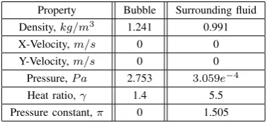
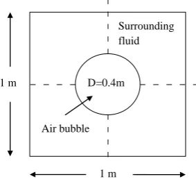
3) Bubble Explosion Under Water Test: This test is also presented in [16] and has been considered by other researchers. The computational domain of this case study including the bubble geometry is illustrated in Fig. 7 and the initial state is shown in table III. The simulation was made using HLL solver and the surface plots for mixture density and pressure are presented in Fig.8.
The numerical results obtained from two dimensional test problems are compared with the equivalent numerical results that published in [14] and [16]. The comparisons are suc-cessful; the current results demonstrate a good compatibility
D=0.32m
Fluid 1
Fluid 2
1 m 1 m
0.25 m
0.25
[image:5.595.99.241.559.633.2]m
Fig. 5. The Flow Domain and the Initial State for the Interface Test
Fig. 6. Volume Fraction Contour (Fig.6a) and Density Distribution (Fig.6b) at Timet= 0.36sfor the Interface Test
TABLE III
INITIALCONDITIONS FOR THEUNDERWATEREXPLOSIONTEST
Property Bubble Surrounding fluid Density,kg/m3 1.241 0.991
X-Velocity,m/s 0 0 Y-Velocity,m/s 0 0
Pressure,P a 2.753 3.059e−4
Heat ratio,γ 1.4 5.5 Pressure constant,π 0 1.505
[image:5.595.332.521.618.705.2]Surrounding fluid
D=0.4m
Air bubble
[image:6.595.102.244.64.193.2]1 m 1 m
[image:6.595.53.289.249.523.2]Fig. 7. The Flow Domain and the Initial State for the Under Water Explosion Test
Fig. 8. Density Evolution (Fig.8a) and Pressure Distribution (Fig.8b) at Timet= 0.58sfor the Under Water Explosion Test
V. CONCLUSION
Numerical simulations of compressible flows between two immiscible fluids have been performed successfully. The nu-merical algorithm for these simulations has been developed based on Godunov approach with HLL and HLLC solvers considering second order precision. The performance of the considered multi-component flow model and the numerical method has been verified effectively. This has been made using a set of carefully chosen case studies which are distinguished by a variety of compressible flow regimes. The obtained results show that the developed algorithm is able to reproduce the physical behaviour of the flow components efficiently. Consequently, it could be applied to simulate a wide range of compressible multiphase flows with different materials and physical properties.
REFERENCES
[1] A. Nowakowski, B. Librovich, and L. Lue, “Reactor safety anlaysis based on a developed two-phase compressible flow simulation,” in Proceedings of the 7th Biennial Conference on Engineering Systems Design and Analysis, vol. 1, pp. 929–936, 2004.
[2] R. Saurel and R. Abgrall, “A multiphase Godunov method for com-pressible multifluid and multiphase flows,”Journal of Computational Physics, vol. 150, no. 2, pp. 425– 467, 1999.
[3] G. Allaire, S. Clerc, and S. Kokh, “A five-equation model for the numerical simulation of interfaces in two-phase flows,”C. R. Acad. Sci. - Series I: Mathematics, vol. 331, no. 12, pp. 1017– 1022, 2000. [4] A. Murrone and H. Guillard, “A five-equation model for the simulation of interfaces between compressible fluids,”Journal of Computational Physics, vol. 181, pp. 577–616, 2005.
[5] A. K. Kapila, R. Menikoff, J. B. Bdzil, S. F. Son, and D. S. Stewart, “Two-phase modeling of deflagration to detonation transition in granular materials: Reduced equations,”Physics of Fluids, vol. 13, no. 10, pp. 3002–3024, 2001.
[6] G. Allaire, S. Clerc, and S. Kokh, “A five-equation model for the simulation of interfaces between compressible fluids,” Journal of Computational Physics, vol. 181, pp. 577– 616, 2002.
[7] J. F. Haas and B. Sturtevant, “Interaction of weak shock waves with cylindrical and spherical gas inhomogeneities,”Journal of Fluid Mechanics, vol. 181, pp. 41–76, 1987.
[8] G. Layes, G. Jourdan, and L. Houas, “Distortion of a spherical gaseous interface accelerated by a plane shock wave,”Physical Review Letters, vol. 91, no. 17, pp. 174 502–1–174 502–4, 2003.
[9] G. Layes and O. Le M´etayer, “Quantitative numerical and experimental studies of the shock accelerated heterogeneous bubbles motion,”
Physics of Fluids, vol. 19, pp. 042 105–1–042 105–13, 2007. [10] F. Coquel, K. E. Amine, E. Godlewski, B. Perthame, and P. Rascle,
“A numerical method using upwind schemes for the resolution of two-phase flows,”Journal of Computational Physics, vol. 136, pp. 272– 288, 1997.
[11] A. Bagabir and D. Drikakis, “Mach number effects on shock-bubble interaction,”Shock Waves, vol. 11, no. 3, pp. 209– 218, 2001. [12] H. Terashima and G. Tryggvason, “A front-tracking/ghost-fluid method
for fluid interfaces in compressible flows,”Journal of Computational Physics, vol. 288, no. 11, pp. 4012– 4037, 2009.
[13] R. K. Shukla, C. Pantano, and J. B. Freund, “An interface capturing method for the simulation of multi-phase compressible flows,”Journal of Computational Physics, vol. 229, pp. 7411– 7439, 2010. [14] E. Toro,Riemann Solvers and Numerical Methods for Fluid Dynamics.
Springer, 1999.
[15] X. Hu and B. Khoo, “An interface interaction method for compressible multifluids,”Journal of Computational Physics, vol. 198, pp. 35– 64, 2004.