Simulating a pay lane within a traffic network using
a choice model based on travel time variability
Masterthesis H. Graaff
October 2008
Twente University
Civil Engineering and Management
Simulating a pay lane within a traffic network using
a choice model based on travel time variability
Masterthesis H. Graaff
Deventer, October 2008
Herman Graaff
Twente University
Faculty of Engineering Technology
Centre for Transport Studies
Student nr
0049867
E-mail address
[email protected]
Thesis committee:
Prof. dr. ir. E.C. van Berkum
Twente
University
Ir.
H.L.
Tromp
Goudappel
Coffeng
B.V.
J.
Zantema
MSc.
Goudappel
Coffeng
B.V.
Preface
This masterthesis is the result of a research about the road user behaviour towards pay lanes. The past months I have worked on this research and with this research I intend to complete my master study Civil Engineering and Management at the University of Twente.
During my research I worked at Goudappel Coffeng. Goudappel Coffeng has a lot of expertise about traffic and transport and a subsidiary of Goudappel Coffeng also developed the software package OmniTrans, that is used to execute the simulations.
I want to thank my thesis committee for their readiness to support my research and invest their time and
knowledge during the research process. I want to thank Goudappel Coffeng for the opportunities they offered me to do this research. I also want to thank Henk Taale for providing the MonicaData and Professor Martin Dijst for his support at the beginning of the research.
Executive Summary
Introduction
The road network in the Netherlands will become more and more congested the upcoming years. Although policy is developed and executed to meet the expected congestion problems, it is expected that the accessibility of some important economic regions in the Netherlands will worsen. The introduction of pay lanes could be a measure to guarantee this accessibility for a share of the road users.
Pay lanes are separate lanes at highways that can only be used by road users that pay a certain toll for it. Pay lanes offer road users an extra service, because at pay lanes a low travel time is guaranteed. Road users are free to choose to use the (congested) free lanes or use the pay lane after paying for a guaranteed low travel time. In the United States several pay lanes have been constructed. Evaluation reports about these pay lanes are very positive. As a consequence of the pay lanes the travel times at the free lanes is improved and road users from all income classes use the pay lanes.
The willingness to pay for a pay lane is caused by both the reduction of travel time and the reduction of travel time variability. A reduced travel time variability gives road users a better indication of their arrival time, what seems to be very valuable for road users that have a great need to arrive on time.
To be able to estimate the potential effectivity of pay lanes in the Netherlands, an estimation has to be made about the valuation of this travel time variability by Dutch road users. Because no pay lane situations are available in the Netherlands, these estimations need to be made with a traffic model in which also the travel time variability has to be incorporated. Therefore the following research objective is formulated:
Research objective:
The objective of this research is to develop a travel time variability based choice model and using this model to simulate two concrete pay lane situations in the Netherlands to get an indication of their effectiveness.
The two concrete pay lane situations are a potential pay lane at the 27 parallel to the Merwede Bridge near Gorinchem and a pay lane at the off-ramp Near Sloten in Amsterdam.
The network model used for the pay lane situations has been taken from the national accessibility model. The national accessibility model is a model developed by Goudappel Coffeng. The road users are divided in the different user classes, which vary in their preferences. The pay lane is added as a separate route in the network. In an iterative procedure the road users are assigned to the road network and subsequently to the pay lane or the free lane.
Simulation results of the pay lane situation at the A27
The congestion that occurs in the old situation is strongly reduced by the pay lane. The congestion effects are fully taken away in the reference situation with three lanes (In the 2020 network this reference situation leads to small congestion effects).
A comparison of the travel costs as a sum of the travel time costs, the schedule delay costs and the toll costs, is shown in the table below. In the individual travel costs the toll costs are included. In the social travel costs, the toll costs are excluded because they are benefited by society as a whole. The pay lane strongly reduces travel costs in comparison with the old situation. At the same time the travel costs for the pay lane are much higher than the reference situation with three lanes, despite the benefits of a guaranteed low travel time.
Travel time costs
Schedule
delay costs Toll costs
Individual travel costs
Social travel costs
2004 – Reference three lanes 29760.49 11122.5 0 40882.99 40882.99 2004 - Pay lane (toll 2,00) 36501.16 10647.9 13385.74 60534.81 47149.06
% - effect 23% -4% 48% 15%
2020 – Reference three lanes 54824.66 23357.25 0 78181.92 78181.92 2020 - Pay lane (toll 3,00) 73772.16 20763.71 30507.66 125043.5 94535.86
% - effect 35% -11% 60% 21%
2004 - Reference two lanes 97221.53 18537.5 0 115759 115759 2004 - Pay lane 36501.16 10647.9 13385.74 60534.81 47149.06
% - effect -62% -43% -48% -59%
In comparison with the pay lane locations in the United States, these pay lane simulations result in a quite low monetary valuation of schedule delay. This can be partly explained by the fact that the used valuation parameters are based on the monetary valuation of a regular schedule delay and not on a stochastic distributed schedule delay. Also the travel time variability is not included as a traffic flow dependent variable within the simulation procedure.
The simulation results show that the addition of a pay lane can reduce the congestion effects at the free lane. In contrary to a regular capacity enlargement, private exploitation of a pay lane can offer a private company return on investment. From this perspective a pay lane seems be an interesting measure to reduce congestion.
It is recommended to investigate the valuation of a stochastic distributed schedule delay in order to be able to make a good comparison between a pay lane situation and a reference situation with a regular capacity enlargement.
Simulation results of the off-ramp near Sloten in Amsterdam
The off-ramp near Sloten has sometimes insufficient road capacity. This results in a queue at the off-ramp and even at the main lanes of the highway. As a consequence on-going traffic is hindered. A pay lane alternative is simulated where a longer ramp is constructed that forms a buffer where road users can wait. The old off-ramp is used as a fast pay lane alternative.
A first test of the pay lane situation results in a total gridlock at the network. This gridlock is the result of a changed route choice by almost all road users that use the off-ramp. Other off-ramps are more attractive than the long new off-ramp or the old off-ramp where toll is charged. This massive changed route choice (which leads to a worse situation for everyone) can also be explained by the modelling structure of OmniTrans. Because route choice is determined in a static traffic assignment and the traffic conditions are determined in a dynamic traffic assignment, road users make the route choice is not based on the occurring traffic situations, but on a much smaller congestion effect that is estimated by the static traffic assignment.
Table of contents
Preface ... 3
Executive Summary ... 4
Table of contents... 6
1. Introduction... 7
2. Background ... 10
2.1 Policy context... 10
2.2 Economical context... 13
2.3 Modelling context ... 16
3. Research questions & methodology ... 23
4. Analysis of travel time variability ... 28
4.1 General description of the used data ... 28
4.2 Statistical analysis of the variation in travel time... 29
4.3 Analysis of the influence of traffic inflow on travel time ... 32
5. The pay lane choice model... 37
5.1 The ideal choice model ... 37
5.2 Assumptions regarding the ideal choice model... 38
5.3 Overview of selected user classes ... 39
5.4 Mathematical procedure of the choice model ... 40
6. The realisation of the two traffic models... 47
6.1 Description of the used software and the basic model ... 47
6.2 Assumptions in the created traffic models ... 48
6.3 The creation of user class specific trip matrices... 49
6.4 Creation and calibration of the two submodels ... 51
6.5 Implementation of the developed choice model within OmniTrans and the submodel structure... 52
7. Situation Bottleneck A27 ... 55
7.1 Properties and assumptions regarding the traffic network ... 55
7.2 Simulated travel times... 57
7.3 Pay lane use by different income classes ... 58
7.4 Traffic conditions at the pay lane ... 59
7.5 Comparison of simulation results pay lane and references ... 61
7.6 Evaluation of simulation results ... 65
8. Situation Off-Ramp Sloten / Amsterdam ... 67
8.1 Traffic network without pay lane ... 67
8.2 Traffic network with pay lane ... 68
8.3 Evaluation of simulation results ... 69
9. Conclusions and recommendations... 70
9.1 Pay lane effects following from the simulations ... 70
9.2 The desirability of pay lanes in the Netherlands ... 71
9.3 Recommendations ... 72
References... 73
Appendix A: Description of speed data sources ... 76
Appendix B: Method for the estimation of the distribution of different user classes in the national model ... 78
1. Introduction
Congestion problems in the Netherlands
The last decennia the car has gained a central position in modern life. The massive introduction of the car has increased individual travel opportunities, but also made people more dependent on their car. In the Netherlands the car ownership and the average distance travelled have increased non-stop during the last sixty years. As a consequence, the number of roads with daily congestion is increasing.
Figure 1: Development of vehicle kilometres (left) and vehicle loss hours (right) on working days, index 2000 = 100 (source: Ministerie van Verkeer en Waterstaat, 2006,II)
The size of this development is shown in figure 1. The left figure shows the (estimated) number of vehicle kilometres for person cars (yellow and light blue) and freight. The right figure shows the number of vehicle loss hours during the morning peak, evening peak and the period between both peaks. Both figures come from a Dutch mobility policy document written in 2006. As can be seen the growth of vehicle kilometres has a more than proportional effect on the congestion size. Also the reliability of travel times decreases. The same Dutch document estimates that the economical loss because of congestion effects will be 2.4 billion euro.
Problems in maintaining the accessibility
The same disproportional effect can be seen in figure 2. The left figure shows the travel time to Schiphol from a certain place in the Netherlands during the morning peak in 2005. The right figure shows the travel times for the year 2020. The area from which Schiphol can be reached within two hours greatly decreases. The figure supports the political concern that a growing congestion has a strong negative impact on the accessibility of important economic regions in the Netherlands, especially the Randstad Area.
Complex policy issue
The congestion problems have created a complex policy issue. The past decennia the enlargement of road capacity led to an increased traffic demand. As a consequence of this, the further enlargement of road capacity is no longer seen as an accurate solution for the expected problems. Also the limited space available near congested roads makes it difficult to make further road improvements. Moreover the negative environmental effects of car mobility were a reason to consider a further growth of mobility as a negative development (Pahaut et al., 2006). For these reasons the past two decades political initiatives are made to introduce a form of road pricing in addition to investments in road infrastructure and public transport. Such taxation can introduce an effective incentive for road users to avoid road use during peak hours. Until 2005 these initiatives did not gain general support for realisation, as a consequence of a lack of confidence in the technical opportunities and the fact that many people interpreted the plans as an extra resource for public funds.
In the year 2005 a group of involved organizations including the government formulated an advice to introduce a general variant of time- and place-dependent road pricing (Nouwen et al., 2005). These new taxes should be compensated by reducing the existing taxes on car ownership. The advice was received positively by the parliament, but several postponements were made the last year in the planning process of the implementation. Even so, during the last year several concrete decisions about the introduction of road pricing were made and during the upcoming years the realization can be expected.
Pay lane: introduction and definition
The road taxation as described in the previous paragraph can be seen as a type of road pricing that deals with all road users. An alternative type of road pricing is the application of pay lanes. In the United States pay lanes have been realized at several places. In pay lane situations a part of the road capacity is allocated to those road users that are willing to pay a certain amount in order to have a guaranteed low travel time.
Scholten et al. (2000) define the following two road pricing mechanisms:
Congestion pricing: Uses road pricing to discourage traffic use during peak hours for all road users.
Value pricing: Uses road pricing to offer road users an additional service that is only available for those road users that are willing to pay toll.
The intended road pricing in the Netherlands can be seen as a form of congestion pricing. Pay lanes are based on the principle of value pricing. Pay lanes intend to guarantee a low travel time for a part of the road users. An additional possibility is to give high occupancy vehicles free access to pay lanes. This can encourage carpooling. The following objective of pay lanes is formulated in an exploring study of the Dutch government:
Presumed that the congestion problems are partially unsolvable, the objective of pay lanes is not to solve all congestion problems, but to maintain the accessibility of certain regions for those road users who are dependent of a good accessibility. Price is therefore the driving decision criterion (Ministerie van Verkeer en Waterstaat, 1999).
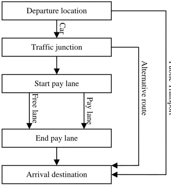
In this thesis a distinction is made between pay lanes and free lanes, which can be defined as following:
Pay lane: Highway lane that offers a guaranteed travel time and which is only accessible for road users who are willing to pay a toll or eventually have free access because they meet other conditions.
Free lane: Highway lane that is situated parallel to a pay lane and that is used by those road users that are not willing to pay a toll and don’t meet necessary other conditions.
Research subject and outline of the report
also describes the most influential factors that determine if road users decide to use the pay lane or the free lane. The third chapter defines the research structure.
2. Background
This background chapter gives an overview of earlier research about pay lanes or related issues. A distinction is made between the policy, economical and modelling context. All these contexts together create the context in which the thesis is executed. Because the thesis focuses on the choice model and not on the physical
implementation of the pay lanes, the technical and physical context of pay lanes is only marginally described in this chapter.
2.1 Policy context
This paragraph considers the policy context of pay lanes. It shows both the situation in the Netherlands, where on a small scale policy initiatives for pay lanes have been started, and the situation in the United States, where pay lanes have been realized.
History of pay lanes in the United States
In the United States most pay lanes are upgraded carpool lanes. These High Occupancy Vehicles (HOV)-lanes were only accessible for cars with two or more occupants. In practice the roads remained almost empty most of the time. As a consequence the social support for maintaining these lanes decreased drastically, the so-called empty-lane syndrome (Scholten et al., 2000). Although in the Netherlands soon after the introduction of the carpool lanes the whole idea was totally cancelled, in California some HOV-lanes were transformed to High Occupancy Toll (HOT)-lanes or Express Toll Lanes (ETL’s). HOT-lanes are both accessible for toll payers and cars with two or more (in some cases three or more) occupants. ETL’s are only accessible for toll payers.
The fairness of pay lanes
The decision to transform the HOV-lanes to pay lanes was not self-evident. At some places the plans failed as a consequence of a negative public opinion. There are several objections towards pay lanes. The first group of objections considers road pricing in general. There is already paid for roads via other taxes, so it is unfair to introduce another tax for the use of it. The second group of objections considers the fact that most pay lane users come from high income classes. By introducing pay lanes these groups gain the most advantages, while for low income classes no measures are taken to reduce their congestion disadvantages. The introduction of the soundbite “Lexus Lanes” seemed to be effective in strengthening the negative public opinion.
To these objections, Litman (1999) makes a clear distinction between horizontal and vertical equity. Horizontal equity considers the extent to which the advantages of a measure are experienced by the one that paid for it. Vertical equity considers the question if people who naturally form the weak groups in society experience an advantage or at least not a disadvantage by a measure.
Baker et al. (1998) have analyzed both aspects for the case of the Californian pay lanes. The article also refers to a stated condition for transport policy by the U.S. government that vertical equity may not worsen by a certain policy measure. In the case of pay lanes the impact on vertical equity depends on the distribution of the pay lane users over the different income classes and the way the toll income subsequently are spent. The pay lane use depends on the valuation of travel time and travel time reliability and for these valuations income is not the most influential variable. The article states that a strong improvement of travel time reliability will make a pay lane attractive for road users spread over all income classes. The connotation of a Lexus Lane is therewith not founded.
The horizontal equity of pay lanes is very strong, because road users have a free choice to pay for the lanes and they directly experience an advantage from it. From this viewpoint value pricing is far more attractive than congestion pricing, where toll payment is unavoidable and no direct visible advantages can be experienced.
Effectiveness of pay lanes in the United States
California State Route (SR) 91
Sullivan et al. (1998) show the results of an evaluation of the effects of the introduction of the pay lanes. An important part of this study is a survey of road user opinions. The most important conclusions:
• Travel times: As a consequence of the extra road capacity of the pay lanes, the travel delay decreased in the first year from 30-40 minutes to less than 10 minutes. The second year the total traffic flow grew and the travel delay increased to 12-13 minutes.
• Vertical Equity: A substantial part of the road users (between 7% and 35% at working days) uses the pay lanes. This percentage is higher for high income groups, but the differences are limited. 25% of the lowest group (< $25.000) versus 50% of the highest group (> $100.000) frequently uses the pay lanes. There is also a significant difference between men (28%) and women (42%).
• Social support: The paylanes can count on a broad social support. Pay lanes as a measure to reduce congestion is supported by 60 – 80% of the respondents. This percentage is 5-10% higher for pay lane users in comparison to non pay lane users. 50-75% supports the private character of the exploitation.
• Carpooling: Although carpooling is no longer the only condition to use the pay lanes, the number of carpooling people at the corridor increased. Baker et al. (2008) suggest this is a consequence of the so-called insurance effect, what means that people are no longer dependent on a co-driver to gain access what makes it possible to maintain the same departure times during the week. This makes carpooling a more attractive alternative.
The I-15 Congestion Pricing Project in San Diego
Another highway road where pay lanes have been successfully realialized is the I-15 near San Diego. Here two physical separated pay lanes are situated that in the morning are accessible in one direction and in the afternoon in the other direction. In this case the toll level is also flexible with a predefined maximum.
Van Amelsfort (1999) studied the occurring travel time and travel time variation at the free lanes of the I-15. At the most congested moment the difference between the median travel time at the free lane and at the pay lane is 6 minutes in the morning and 3,5 minutes in the afternoon. Also the travel time corresponding to the 90th percentile is calculated as an indicator of travel time variability. Here the difference at the heaviest peak moment is 10 minutes in the morning and 16 minutes in the evening. Van Amelsfort also reports that the traffic flow is increased as a consequence of the addition of the pay lanes with a yearly 20% during the first two years. An analysis of the pay lane users shows that the total travel time and the gender of the road user have a strong relationship with the share of pay lane use.
Another interesting finding of the study is the impact of the flexible toll level. When the travel time at the free lane is relative high, the toll level is set high in order to prevent too many people use the pay lane. When the travel time at the free lane is relative low, the toll level is set lower so that more people use the pay lane and the lane does not stay empty. When the assumption is made that road users compare the costs and the benefits of using the pay lane, it is expected that a lower toll level encourages more people to use the pay lane. But in practice this flexible toll is seen by road users as an indicator of the travel conditions at the free lane. So a high toll level means that it is necessary to use the toll to arrive on time, while a low toll level shows that the free lane can be used without congestion. This effect emphasizes the problem of keeping the pay lane an attractive service in different situations. The flexible toll level seems not to be an accurate solution for this problem.
Potential social support in the Netherlands
The evaluation results of the pay lanes in the United States nuance the view that pay lane use is mostly related to income. Pay lane use is higher for high-income groups, but pay lanes are used by all income classes, especially to reduce travel time variability. In The Netherlands this perception of pay lanes within political debate and public opinion usually lacks this nuance. In the previous decade several studies are made about the possibilities of pay lanes in the Netherlands. The broadly supported advice to introduce general road taxation (see also the previous chapter) did not include pay lanes and as a consequence the discussion about pay lanes was only marginally continued. Despite it is interesting to state the most important findings of these studies.
In 1998 a study is made about the opinion of several involved organizations towards pay lanes (Ministerie van Verkeer en Waterstaat, 1999). The study shows that consumer organisations and the Dutch Chamber of Commerce prefer pay lanes above congestion pricing. Other organisations consider pay lanes as a good
supplement to other pricing measures. Aarnink (1998) confirms this view that many involved organizations have a positive view towards pay lanes. Also a broad consensus exists about the criterions for these pay lanes:
• Choice freedom for the road user
• No exclusion of road users (e.g. carpoolers) from payment
• Guaranteed low travel time at pay lane
• Pay lanes are created as extra lanes
• Toll level is variable
• Pay lanes can be exploited by a private organization
Other studies show the influence of the destination of toll revenues for the social support towards forms of road use taxation. A study of Verhoef (1996) shows that this aspect is crucial for 83% of the road users in the Netherlands. Small (1992) shows that public and political support increases as the direct effect of a tax payment (e.g. a reduced travel time) is larger. The guaranteed travel time can therefore be seen as the most important advantage of a pay lane in comparison with congestion pricing for the acquiring of social support. Parry and Bento (2001) show that a general welfare gain can be achieved when toll costs are compensated by a reduction of taxes with a disturbing effect on the labour market. Lumpsum compensation towards households seems significantly less effective.
Ubbels (2005) has studied the degree of acceptation of different ways to use toll revenues. At a scale from 1 (very unacceptable) to 7 (very acceptable) the following alternatives are judged by respondents:
• General budget (2,15)
• Lower income taxes (3,86)
• Improvements in public transport (3,99)
• Construction of new roads (5,20)
• Lower fuel taxes (5,58)
• Lower taxes for car ownership (5,84)
Beside the social support also the physical opportunities to create pay lanes in the Dutch road network and the limited space for capacity increasement in the cities are studied. DHV (1997) studied a dual system where in the whole Randstad Area both a free lanes and a pay lanes network are created. The study shows that several bottlenecks have to be solved, including some very complex cases. Another study (Ministerie van Verkeer en Waterstaat, 1999) shows a number of separate potential pay lane locations. The study concludes that in most cases a combination of a general capacity enlargement at a part of the section and a pay lane realisation on the remaining part of the section is desired. This offers as much as possible traffic to use the pay lane and at the same time the pay lane is prevented to get hindred by congestion when the pay lane starts before the point where congestion starts.
Another aspect that can postively influence the opportunities for pay lanes in the Netherlands is the private exploitation of pay lanes. One of the current problems with respect to investments in new road infrastructure is the limited budgettary space for these kinds of investments. Some investments will result in far more economical benefits than costs, but as a consequence of too high costs for building these investments are not made. When the opportunity is offered towards a private organization to acquire the ownership of a pay lane after financing and building it this problem could be tackled. Because the pay lane is an additional alternative for road users, there is no problem of a monopolistic ownership, one of the occurring problems at general forms of private road
ownership.
2.2 Economical context
The second context of this thesis is the economical context. The effects of road pricing measures usually are expressed in economical terms in order to analyse their effectivity. It is important from which perspective this economical analysis is executed. It could for example be possible that a private organisation that exploitates a road gets a great profit out of this exploitation, but at the same time many road users are financially
disadvantaged by the high tolls. For that reason economical analyses usually are based on the evaluation of gains and losses for society as a whole. Most of the times, not only real monetary profits and losses are incorporated, but also non-monetary profits and losses like travel time and environmental effects are monetarised. In this paragraph an overview will be given of the economical context of pay lanes as stated in earlier research.
Marginal cost pricing
The idea of congestion pricing as an effective congestion reducing method is based on the principle of marginal cost pricing. This principle can be shown using an economical model for a situation where one road is available between a certain origin and a certain destination. There is an amount of car travellers that like to use the road to travel from the origin to the destination.
The costs to use the road depend on the number of road users at the road. As this number increases, the travel time also increases as a consequence of congestion effects. In general, these costs as a function of the number of road users vacan be estimated using the following formula (Small et al., 2000):
) ( )
( a a a
a v L t v
c =β⋅ +α⋅ (1)
Where further L is the length of the road and ta(va)the travel time corresponding to the number of road users.
α and β are parameters for the monetary valuation of distance and time. Usually congestion effects become stronger as the number of road users nears or exceeds the road capacity. Figure 3 shows a possible cost function for the road as a function of the number of road users.
At the same time all road users have a certain welfare gain for making the trip. This welfare gain differs for each road user. Road users only make a trip when this welfare gain is larger than the trip costs. When trip costs are larger than the welfare gain, road users could better stay home. As a consequence the demand for using the road decreases as the costs for using the road increase. This leads to the demand line in Figure 3.
Figure 3: Economical model for a road (source: Yang et al., 1998)
Following the economical principles this situation leads to the equilibrium situation that has been marked with A in the figure. Despite the reached equilibrium, this is not an optimal situation. The first reason is that external effects towards the environment are not incorporated by the cost function. The incorporation of these costs is usually aimed by fuel taxes or general road taxation (Mankiw, 2001).
congestion effects of this user towards all other road users. These marginal social costs can be described using the following formula (Yang et al., 1998):
a a a a a a a a
dv v dc v v c v
c ( )= ( )+ ( ) (2)
Where the first term represents the costs experienced by the new road user and the second term represents the changed road costs by this adding of a road user towards all other road users. The optimal equilibrium situation would be the situation in which these marginal social costs are equal to the marginal welfare gain (point B in the figure). This could be reached by introducing a toll with a price equal to the line HB in the figure. This makes the cost function move upwards and intersect the demand function in point B. This toll can be estimated using the following formula:
a a a a
dv v dc v ( )
=
τ (3)
Optimal tolls within a network
Within a traffic network usually more than one route is available between two places. As a consequence it could be possible that when a toll based on the marginal cost pricing principle has been introduced at one of the routes, road users will switch route and use a road where marginal costs are not priced. This situation could be less optimal than the old situation. To really reach an optimal situation in which all marginal social costs are incorporated in the costs a road user experiences, it is therefore necessary that on all routes in a network a toll is charged to incorporate the marginal costs. When this situation is realised, this is called the first best (FB) optimum (Williams et al., 2001).
In practice it is quite difficult to apply marginal cost pricing on all roads in a network. Usually toll charging is limited to highways. The situation that road users switch to local roads to avoid toll charging is strongly undesirable. In such a case it is better to charge a much lower toll. This lower toll optimum is called the second best (SB) optimum, because the optimum is constrained by a number of no-toll routes in the network.
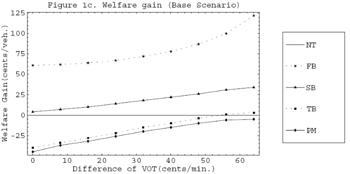
Next to the first best and second best optimum, there is also a third best (TB) optimum. This optimum is not only limitated by a number of no-toll routes at the network, but also by the condition that the number of vehicles at the toll road must be lower than for example 80% of its capacity, in order to guarantee a certain level of service. This second condition leads to a less efficient use of road capacity at the pay lane and this leads to a situation that is less optimal than the second best optimum. The principle of pay lanes can be seen as a TB optimum. Small et al. (2000) have simulated a FB, SB and TB optimum for a network with one origin, one destination and two possible routes. The simulation is based on two user groups with each a different value of time. The difference between the values of time of both groups is varied between 0 and 70 cents per minute. For each situation the welfare gain under no toll conditions is determined. Subsequently the welfare gains under FB, SB and TB conditions are determined and these are related to the no toll situation.
Figure 4: Results of a two route simulation for two user classes and several value of time differences
The effectivity of pay lanes in relationship to congestion pricing
The results shown in the previous paragraph indicate that the condition of a guaranteed low travel time leads to a welfare loss. Based on these findings, the conclusion could be drawn that a general variant of congestion pricing is a better measure than the creation of pay lanes. Despite these results, pay lanes have other advantages that can improve the welfare gain, but are not incorporated in this analysis.
The most important advantage of TB-pricing is that travel time uncertainty is reduced for pay lane users. As a consequence costs resulting from arriving too early or too late will be much smaller than when a road user uses a free road or a toll road under SB conditions. The next paragraph describes the valuation of these travel time reliability.
Another advantage of TB-pricing is that there could be a substantial external valuation for a guaranteed
2.3 Modelling context
The third context is the modelling context. As described in the previous paragraphs, a pay lane can offer a reduction in travel time and also a reduction in travel time variability for those road users that are willing to pay a certain toll. This paragraph gives an overview of earlier research about the measurement and valuation of travel time variability.
Travel time variability and schedule delay
A reduction of travel time variability is seen as a significant advantage offered by a pay lane. This means that a disutility is experienced by a road user as a consequence of travel time variability. But what are the causes of these costs? And how can these costs be related to the other occurring costs?
Noland et al. (1997) give an overview of different ways in which travel time variability costs are incorporated in cost functions. There is a main distinction between two aspects that lead to these travel time variability costs:
• Disutility due to congestion:
Travel time variability usually is a consequence of congestion. Congestion leads to a larger travel time and also to a larger discomfort in comparison to free flow conditions. Both aspects lead to a certain disutility.
• Disutility due to schedule delay:
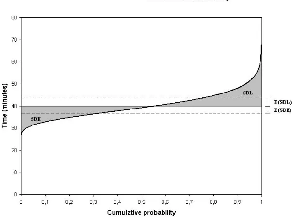
As a consequence of travel time variability there is a strong probability that a road user arrives too early or too late at the destination location. When a road user has an important appointment, he can reduce his probability on arriving too late by choosing an earlier departure time. Usually this safety margin leads to an ineffective period spent at the destination location. Arriving too early and arriving too late almost always result in a disutility which is defined as schedule delay costs early (SDE) or schedule delay costs late (SDL).
For both aspects the size of the disutility is related to the level of travel time variability. An important difference is that the first aspect considers costs that are related to the characteristics of the trip itself, while the second aspect considers costs that are related to the purpose of the trip.
When the travel time variability is assumed to be a certain stochastical distribution, the occurring travel time can be estimated for different probabilities. For example the 80% travel time is the travel time that is higher than 80% of the registrated travel times. The valuation of the disutility due to congestion is mostly based on the difference between the travel time in a congested situation (for example the travel time for which 80% or 90% travel time) and the median or average travel time. This leads to the following cost function:
( )
C =α⋅t50%+β⋅(
t90%−t50%)
+τE s (4)
Where t50% is the median travel time and t90%the 90% travel time. αand β are valuation parameters for travel
time and congestion. τis the toll level.
The valuation of the disutility due to schedule delay is based on a similar stochastic distribution, but this first has to be translated to an expected schedule delay early and late. This leads to the following cost function:
( )
C =α⋅E(T)+β⋅E(SDE)+γ⋅E(SDL)+τE s (5)
Where E
( )
T is the average travel time, E(
SDE)
and E(
SDL)
are the expected schedule delay early and late andβ
α, and γ are valuation parameters for travel time and schedule delay. It is also possible to add a penalty to the cost function that is calculated once when a road user arrives too late. This describes a disutility that is a consequence of arriving too late, but that does not depend on the size of the delay.
This means that in the first formula the valuation of the schedule delay disutility is incorporated in the parameter
β and in the second formula the valuation of the congestion disutility is incorporated in the parameters β and
γ .
The underlying principle of schedule delay
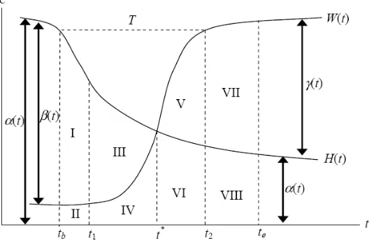
Tseng et al. (2007) show the underlying principle of schedule delay. In figure 5 the utility experienced at work
( )
tW and at home H
( )
t are described during the morning. Because first the utility at home is larger than the utility at work and later vice versa, a road user plans his trip around the switch moment and in such a way that the missed utility during the trip is as small as possible.Suppose a trip has a duration of T as shown in the figure. The chosen departure time tb is the most optimal, because during the period between tb and t2 the available potential utility is smaller than before and after this
period. The total disutility is the same as area I till VI in the figure. When the occurring travel time is lower (for example tb to
*
[image:17.595.99.368.355.529.2]t ) the total disutility is lower (area I, II, III and IV). The occurring utility is increased with area V and VI, but as can be logically deduced from the figure, this utility would be larger when a later departure time is chosen and less utility at home would be lost. For a situation with a larger travel time the figure similar shows that an additional disutility occurs, that would be smaller when an earlier departure time is chosen. The relative utility at home during the early morning β
( )
t and the relative utility at work during the late morning γ( )
t determine this lost utility due to schedule delay.Figure 5: Underlying principle of schedule delay (source Tseng et al., 2007)
Estimation of parameters
The parameters in the cost functions described in the previous paragraphs determine the influence of the different elements on the resulting costs. Different studies are made about these parameters and the influence of socio economic factors on them. For these studies there is a main distinction between Revealed Preference (RP) studies and Stated Preference (SP) or stated choice studies. Both studies will be described separately in the next paragraphs.
Usually both studies have been based on a logit model. Within a logit model for each user i and alternative j the systematic utility or disutility Vij is estimated based on all K relevant attributes Xik and the (unknown) parameters βik using the following formula (Tseng et al., 2005):
∑
=
= K
k ik ik
ij X
V
1
β (6)
Assumed there is a stochastic variation εij between this systematic utility for the different users, the utility Uij is estimated using the formula:
J j V
Based on this stochastic variated utility function, the probability a traveller i chooses to use alternative j can be described as:
∑
= = = J j ij ij i V V j Y P1exp( )
) exp( )
( (8)
When data are available about the resulting distribution of users between the different alternatives and the corresponding values of the attributes, the parameters βik can be found for which the resulting distribution of users from the logit model correspond to the distribution found in the data. This is done by maximising the likelihood, which is described by the following formula:
∑∑
= = = = n i J j i ij PY jd L 1 1 ) ( log log (9)
Where dijis the proportion of the road users that chose for alternative j. When the most likely parameters ik
β have been determined, the monetary valuation of each attribute can be calculated by dividing this parameter by the parameter that corresponds to the monetary costs (for example toll). The value of time for example is calculated by the following formula:
C T dC dU dT dU VOT β β = = / / (10)
The value of reliability (for example expressed as the difference between t90% and t50%) can in a similar way be
calculated by the following formula:
C R dC dU dR dU VOR β β = = / / (11)
Revealed Preference
Revealed Preference studies are based on data available from an existing mobility situation. Interviews or loop detector data are used to determine the occurring distribution of travellers between the different alternatives. Based on this distribution the most likely parameters are estimated with which the choice distribution resulting from the choice model corresponds to the occurring distribution.
Lam and Small (2001) studied the preference at the SR-91. 389 respondents were asked during what share of their trips they use the pay lane. Also some socio economic characteristics like gender and income are
registrated. The Value of Time and Value of Reliability have been estimated using different choice models. The resulting Value of Time is $ 19.22 / hr. The resulting Value of Reliability (with reliability expressed as the difference between t90% and t50%) is $ 11.90 / hr for men and $ 28.72 / hr for women. This significant difference
is explained by the fact that women seem to have more time restrictions and are more willing to pay for saving time. The results further show that the Value of Time is dependent on the total trip length (variations between $5 / hr and $26 / hr).
Brownstone et al. (2003) made a similar study about the pay lane use at the I-15 using an interview among 684 respondents. A share of this group is FasTrak user, another share is carpool driver and the remaining
respondents are free lane users. Because the toll level at the I-15 is flexible, the expected toll and its variance is determined. Based on these a logit model is constructed with a large number of attributes. Using this logit model the Value of Time is estimated to be $ 30.98 / hr for commuters and $ 71.07 / hr for non-commuters.
In another article Brownstone and Small (2005) compare different studies about the Value of Time and the Value of Reliability at both pay lane locations with each other. The different results show an average Value of Time between $ 20 / hr and $ 30 / hr. Further the estimation is done that two third of the quality difference between the pay lanes and the free lanes can be declared by the reduction of travel time and one third of the quality difference by the reduction of travel time variability.
this reason in some studies the interaction between the actual toll level and the travel time variability is included during the determination of the Value of Time. As a consequence it becomes very difficult to make an accurate estimation of the Value of Reliability. The article therefor considers all estimations that have been made about the VOR of the I-15 unreliable.
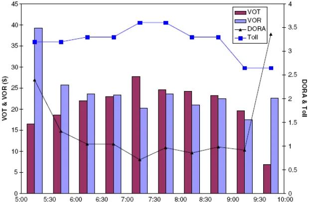
[image:19.595.87.398.251.454.2]An alternative method for the determination of the Value of Time and Value of Reliability is described by Liu et al. (2007). In this method loop detector data are used. A consequence of this method is that segmentation of the measurements based on socio economical data is not possible. With these data an estimation is made of the travel times during morning time intervals of 5 minutes at the SR91. For each time interval the median travel time and the 80% travel time is determined. For the same time intervals the distribution of vehicles between the pay lanes and the free lanes is determined. These data are applied together in a simple logit model containing the attributes travel time, travel time variation and costs. For each 30 minutes the Value of Time and the Value of Reliability is estimated using the most likely parameters. Further the Degree Of Risk Aversion (DORA) is calculated as the Value of Reliability divided by the Value of Time. The resulting values are shown in figure 6.
Figure 6: Estimation of Value of Time and Reliability SR91 based on loop detector data (Liu et al., 2007)
Stated Preference
In Stated Preference studies a fictive travel situation is used to determine the parameters for the different attributes. Respondents are asked to select their favourite travel alternative out of different options and based on this choice the valuation of the attributes is estimated.
The most important difference between Stated Preference and Revealed Preference is that SP studies are based on fictive situations, while RP studies are based on real situations. An important advantage of SP is that it is very easy to vary the travel situation for which the preferred travel alternative has to be selected between different respondents. This makes it possible to make a more clear distinction between the influences of the different attributes. RP studies are usually based on one occurring (average) travel situation and this makes it more difficult to determine what part of the valuation of an alternative can be explained by for example travel time reduction, what part by travel time reliability and what part by a reduction of expected schedule delay (Liu et al., 2007).
An important disadvantage of SP is that it estimates the valuation based on a fictive situation. Respondents could make other choices in real situations. This is related to the fact that in real situations no full information is available about the (expected) trip characteristics. If a traveller has little time or a traveller has adjusted his daily schedule pattern, he could have a significantly different valuation for different attributes. Another disadvantage is explained by the perception of travel time reliability. Noland and Polak (2001) state that this perception could be different from the occurring travel time reliability.
For Dutch travellers several SP studies have been executed. Van Amelsfort and Bliemer (2005) have studied the valuation of travel time variability in terms of schedule delay. They have also added an uncertainty term to equation 5. This is done because in some situations the median travel time is almost the same as the free flow travel time, while the occurrence of incidents ans sometimes congestion result in very high travel times. These irregular high travel times lead to a large extra travel time, but this travel time is not incorporated in the expected travel time or expected schedule delay.
Tseng et al. (2005) have studied the valuation of time and schedule delay for Dutch commuters. This SP study has been used to estimate valuation parameters within this study. This study is described in chapter 5.
Incorporation of travel time variability in a traffic simulation procedure
Within a traffic simulation procedure, traffic is assigned based on a certain assignment logarithm. Within this logarithm all relevant attributes are incorporated. When these attributes depend on the assignment results, usually these logarithms have an iterative structure in which the relation between assigned traffic and the attribute is incorporated.
A frequently used relationship between traffic flow and travel time at a road is the so-called BPR-function. This function describes the travel time ta as a function of the traffic flow vawith the following formula (De Dios Ortúzar et al., 2001):
⎥ ⎥ ⎦ ⎤ ⎢ ⎢ ⎣ ⎡ ⎟⎟ ⎠ ⎞ ⎜⎜ ⎝ ⎛ ⋅ + ⋅ = k a a a C v t v
t ( ) 0 1 γ (12)
Where t0is the travel time under free flow conditions, Cis the capacity of the road and γ and k are roadtype
specific parameters. This function is able to estimate the average travel time at a road under certain circumstances, but does not describe the travel time variation that occurs.
Therefore Tu et al. (2008) have described a method to estimate travel time variability. In the article the assumption is made that above a certain occurring traffic inflow there is a probability that a traffic breakdown occurs. This makes the travel time instable. For this reason the travel time unreliability (TTUR) can be described as a function of the travel time variability under normal conditions (TTVf) and under breakdown conditions
( j
TTV ) using the following formula: j br r f br
r TTV P TTV
P
TTUR=(1− )⋅ + ⋅ (13)
Where Prbr is the probability a traffic breakdown occurs. When sufficient data are available, all elements in the formula can be made dependent on the traffic inflow qin:
) ( )) ( 10 ) ( 90 ( )) ( 1 ( )) ( 10 ) ( 90 ( )
(qin TT thf qin TT thf qin Prbr qin TT thj qin TT thj qin Prbr qin
TTUR = − ⋅ − + − ⋅ (14)
Where TT90thand TT10thare the travel times with a 90% and 10% cumulative probability.
Although this method gives a procedure to describe travel time variation as a function of traffic inflow, a strong inconsistency of the method is that it uses two separate differences. Suppose under normal condition the difference between the 90% and 10% cumulative probability for normal situations is 5 minutes and the
difference between the 90% and 10% cumulative probability for breakdown situations is also 5 minutes, but the average here is 15 minutes larger. Then the TTUR would be 5 minutes according to the formula. This result seems to a very bad indicator of TTUR, because the real difference between the !0% lowest and 10% highest travel times is more than 15 minutes.
The influence of accidents
Incidents usually have a small probability to occur, but when they occur, travel times could be very high. Cohen and Southword (1999) describe a method to estimate the delay after incidents as a function of the V/C ratio, the share of road capacity that is used.
i
T rC V
Q=( − )⋅ (15)
Where V is the traffic flow, rC is the reduced road capacity that is available after the incident and Ti the duration of the blockade at the incident location. After the blockade is taken away, the queue dissolves after time period Tg that is calculated using the following formula:
) /(gC V Q
Tg = − (16)
Where gC is the getaway road capacity. After some mathematical operations this leads to the following formula for the total delaytime:
) / /( ) )( / ( ) 2 / 1
( C T2 V C r g r g V C
D D
D= i+ g = ⋅ ⋅ i ⋅ − − − (17)
The different types of incidents that can occur are classified in the article. The assumptions are made that the probability of an incident can be described by a Poisson distribution and the duration of an accident by a γ -distribution. With these classifications and assumptions general equations are made for the mean and variation of the incidence delay as a function of the V/C-ratio. For example for a freeway with two lanes in each direction the following mean μd and variation
2
d
σ of delay d are estimated:
07 . 4 2 . 21 2 93 . 3 7 . 18 ) / ( 00199 . 0 ) / ( 00408 . 0 ) / ( 00446 . 0 ) / ( 0154 . 0 C V C V C V C V d d ⋅ + ⋅ = ⋅ + ⋅ = σ μ (18)
The method is useful bacause it is based on a microscopic analysis of incident delays and translates these delay to a mean and variation of travel time. But before applying the method the importance of incidents towards the congestion problem has to be evaluated. Mostly incidents lead to such a high travel time and they occur such little that it is nearly impossible to incorporate the potential incident delay in a schedule time margin.
Applying travel time reliability in cost functions
Shao et al. (2006) describe a model in which the user equilibrium is not based on travel time but on travel time variability. This equilibrium is called the Demand driven travel time reliability-based user equilibrium (DRUE). Within this DRUE all road users make their route choice by minimising the costs ca as the sum of travel time
a
t and a safety marginsa: ) ( ) ( )
( a a a a a
a v t v s v
c = + (19)
Where both the travel time as the safety margin are dependent on the traffic flow at a certain road va. In the article this safety margin is chosen in such a way that there is a 95% probability on arriving on time and the assumption is made that the traffic inflow can be described by a normal distribution. The travel time taas a function of the traffic inflow va is described by the following formula:
a a a a a C V t V
t ( )= 0 + (20)
Where t0a is the travel time under free flow conditions and Ca the road capacity. Using these assumptions formula 19 can be rewritten as:
a a a a a a t a a a C V C V t t v
c ( )= +1.65⋅σ = 0+ +1.65⋅cov⋅ (21)
And the covariance can be calculated using traffic inflow q and variation σq:
q
q
σ =
For a two road network with a highway and a local road the normal user equilibirum (UE), the probit stochastic equilibrium (Probit SUE) and the DRUE have been estimated. The conditions of these equilibriums are shown in Table 1.
UE Probit-SUE DRUE
Highway Local road Highway Local road Highway Local road
Average traffic inflow 100,00 < 175,00 116,04 < 158,96 154,21 > 120,79 Average travel time 2,25 = 2,25 2,29 > 2,09 2,39 > 1,71 Reistijd SD 0,13 < 0,87 0,15 < 0,79 0,19 < 0,61 Veiligheidsmarge 0,21 < 1,44 0,24 < 1,31 0,32 < 1,00 Effectieve reistijd 2,46 < 3,70 2,53 < 3,40 2,71 = 2,71
Table 1: Simulation results of three different user equilibriums (Shao et al., 2006)
Because the travel time at the local road increases much faster as traffic flow increases, the necessary safety margin at the local road is larger than at the highway. For this reason in the DRUE more traffic inflow is assigned to the highway in comparison to the UE and the probit-SUE.
3. Research questions & methodology
In the previous chapter the background of pay lanes from different perspectives is described. This chapter describes the research structure. First the main problem is defined as a summary of the first two chapters. Secondly the research questions and objectives are stated. Finally the research methodology is described.
Problem definition
The road network in the Netherlands will become more and more congested the upcoming years. To meet the rising problems, policy is developed to increase road capacity at several places and to introduce a general congestion charge to discourage road use during peak hours.
An alternative or complementary policy instrument is the introduction of pay lanes. This introduction was considered at the end of the last decade, but is not implemented in the transport plans, due to a lack of political support. In the United States several examples of pay lanes are available. In most situations the pay lanes provide a valuable alternative for the free lanes. Pay lanes possess broad social support and increase the accessibility of congested areas for those users that are highly dependent on this.
Pay lanes could also be a valuable policy instrument to maintain the current level of accessibility in the Netherlands. To create social and political support for pay lanes in spite of the current negative opinions it is essential to have a good insight in the likely congestion effects before. Therefore accurate traffic simulations are necessary.
At this moment there is very limited experience with the simulation of pay lanes in traffic models. The choice behaviour that occurs differs strongly in comparison to regular freeways, because not only travel time, but also travel time variability varies very strong. Based on this lack of experience, the following problem statement can be defined:
Problem statement:
The monetary valuation of pay lanes in the United States is for an important part based on the valuation of travel time reliability. There is a strong uncertainty about this valuation of Dutch road users and the way this aspect can be incorporated within a choice model. This makes it difficult to accurately forecast the congestion effects of pay lanes.
Research questions
In addition to the problem statement, the following two research questions are formulated:
1. How can a travel time variability based choice model for a pay lane be composed and integrated in a traffic network simulation procedure?
2. What indicative conclusions can be derived from the simulation of two concrete pay lane situations with respect to the opportunities for introducing pay lanes in the Netherlands?
Because both questions are quite generally formulated, there are also stated several sub-questions. The following sub-questions correspond to the first research question:
1.1 What Travel time variability can be deduced from available loop detector data for the present situation and is it possible to estimate the relationship between traffic inflow and travel time variability based on these loop detector data?
1.2 How can the travel time variability be integrated in a cost function of a pay lane choice model? 1.3 How can this pay lane choice model be implemented in a simulation procedure for a traffic network? 1.4 What limitations has the used software for executing an accurate pay lane simulation?
And the following sub-questions correspond to the second research question: 2.1 What are the congestion effects of adding a pay lane?
2.2 How are the users of the pay lane expected to be distributed between the different income classes? 2.3 To what extent is the pay lane able to guarantee a high level of service under different traffic conditions
in the road network?
Research objective
The objective of the research is to develop a travel time variability based choice model and simulating this model within two concrete pay lane situations in the Netherlands to get an indication of their effectiveness.
Research methodology
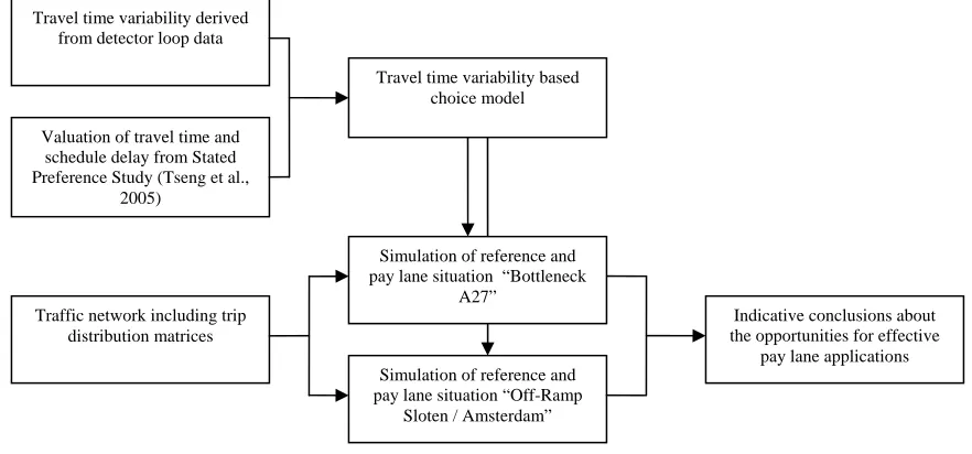
[image:24.595.66.507.180.386.2]Based on these research questions and the corresponding research objective, a research model is constructed. This model is shown in figure 7. The structure of this thesis corresponds to the different elements of the research model.
Figure 7: Research Model
Input elements
The research model contains three input elements. Each element will now be shortly described. With these input elements two main methods have been applied. These two methods will be described afterwards.
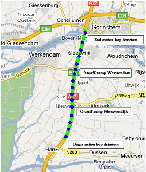
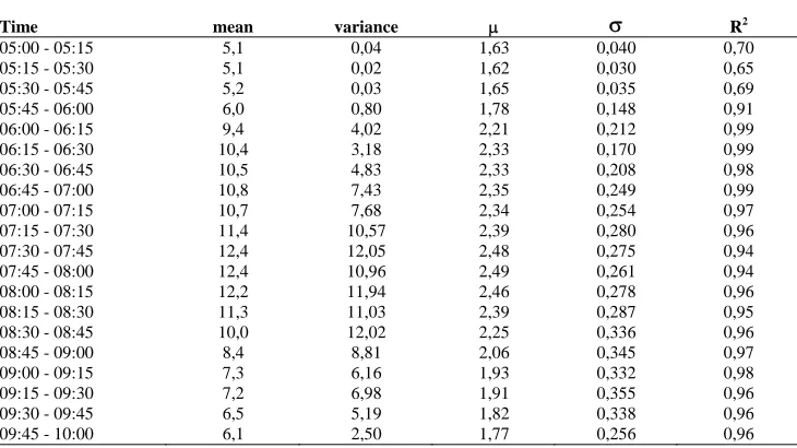
Travel time variability
The travel time variability is an important component of the developed choice model. For this reason an analysis of the occurring travel time variability at the A27 bottleneck (one of the two pay lane situations) is executed. This analysis is described in chapter 4. The results of this analysis are used in the choice model.
Valuation of travel time and schedule delay
As described in chapter 2, Stated Preference studies are useful to estimate the valuation of travel time and schedule delay for different road users. The results of the Dutch research described by Tseng et al. (2005) are considered and translated to the modelling context in order to get proper valuation parameters in the choice model. This is described in chapter 5.
Traffic network and trip distribution matrices
The two case studies are simulated with a representative traffic network. For both simulations this network is deduced from an existing national accessibility model and a corresponding number of trip distribution matrices. This model is described in chapter 6.
Method 1: constructing a choice model
One of the current main problems in simulating a pay lane situation is the estimation of the pay lane use. The proportion of the road users that decide to use the pay lane determines the level of service on both the free lanes and the pay lane. As stated in the introduction, price is the most important criterion for people to decide to use the pay lane. Therefore in this research a choice model is constructed that expresses the experienced advantages of the pay lane use in terms of money.
As stated in chapter two, a pay lane with a guaranteed travel time not only offers an improved travel time, but also significantly reduces the risk for road users to arrive too late or too early because the travel time variation is very small. This effect is much smaller within regular traffic simulations. For this reason in this research these pay lanes are not simulated by a regular link-cost (travel time) optimization procedure, but a separate choice model is applied to estimate the proportion of pay lane users. The expected schedule delay depends on the
Valuation of travel time and schedule delay from Stated Preference Study (Tseng et al.,
2005)
Travel time variability derived from detector loop data
Travel time variability based choice model
Traffic network including trip distribution matrices
Simulation of reference and pay lane situation “Off-Ramp
Sloten / Amsterdam”
Indicative conclusions about the opportunities for effective
pay lane applications Simulation of reference and
occurring travel time variation. For an accurate estimation of this variation, an analysis of detector loop data is executed.
Because the monetary valuation of travel time and schedule delay also differs for each road user, there is also made a distinction between different income groups and within these income groups between road users with high schedule delay costs and users with low schedule delay costs. And because the schedule delay also depends on the real travel time before and after passing the pay lane section, there is made distinction between small trips and long trips.
This leads to the following components of the choice model:
• Toll
• Expected travel time pay lane / free lane section
• Expected schedule delay early
• Expected schedule delay late
• Expected travel time before and after pay lane / free lane section
For the application of the choice model the following differentiations will be made:
• Time of day
• Income class
• Sensitivity for schedule delay
• Possible compensation for pay lane usage by employer
• Trip length
• Toll level
The construction of the choice model is described in chapter 4.
Method 2: Simulation of two possible pay lane situations
After the construction of the choice model two possible pay lane situations are simulated. These simulations are considering a traffic network where for one section a pay lane is provided as an alternative. For this simulation the developed choice model is implemented in the traffic simulation procedures. Chapter 5 and 6 describe this procedural implementation. Chapter 7 and 8 show the concrete construction of the pay lane and the simulation results of both situations. Now the both situations are shortly described.
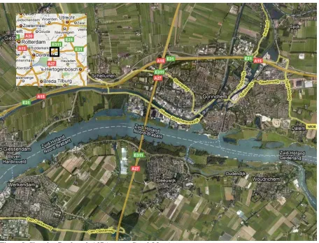
Situation “Bottleneck A27”
The first situation is the bottleneck at the A27. This bottleneck is a consequence of the Merwedebridge that crosses the Waal River near Gorinchem. The capacity of the road at the bridge is smaller than the capacity of the highway track elsewhere. The main reasons for this difference are the absence of a shoulder lane and the smaller width of the two lanes. Although there is no reduction in the number of lanes, there are great congestion effects at the bridge during peak hours. In the morning peak congestion occurs for the traffic travelling to the north and in the afternoon peak congestion occurs for the traffic travelling to the south.
Figure 8: Situation Bottleneck A27 (source: GoogleMaps)
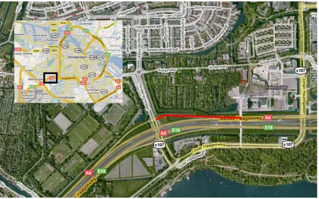
Situation “Off-Ramp Sloten / Amsterdam”
The second situation is the off-ramp near Sloten in Amsterdam. During the morning peak congestion occurs at this off-ramp as a consequence of the waiting time at the junction at the end of the off-ramp. At some times the resulting queue is longer than the off-ramp. This means that also the on-going traffic at the Ring of Amsterdam has an impedance by the off-ramp. As traffic flows grow the upcoming years, it is possible that on several places at the Ring junctions at the end of off-ramps negatively influence the traffic conditions at the highways.
A potential solution for this problem is the creation of extra road length at the off-ramp. As a consequence the waiting times at these off-ramps could increase further, but the negative effects for the on-going traffic are taken away. In this situation a pay lane is created as a fast alternative for the extra long off-ramp. On this pay lane road users can leave the Ring at a high speed and don’t have to wait at the off-ramp.
This pay lane variant is simulated for the off-ramp near Sloten. Figure 9 shows the current situation. The red line is the off-ramp for which the adapted situation is simulated. The reference situation considers only the
Figure 9: Situation Off-Ramp Sloten / Amsterdam (source: GoogleMaps)
Evaluation of simulation results
The last step in the research model is the evaluation of the simulation results. Corresponding to the research sub-questions, several aspects of the simulation results are analysed:
• Social distribution of pay lane users (high / low income classes)
• Travel time of the pay lane for different circumstances
• Congestion costs in comparison to reference situation