Solving Limited-Memory BFGS Systems
with Generalized Diagonal Updates
Jennifer Erway,
Member, IAENG,
and Roummel F. Marcia,
Member, IAENG
Abstract—In this paper, we investigate a formula to solve systems of the form (Bk+D)x= y, where Bk comes from a limited-memory BFGS quasi-Newton method and D is a diagonal matrix with diagonal entries di,i ≥ σ for some
σ > 0. These types of systems arise naturally in large-scale optimization. We show that provided a simple condition holds on B0 and σ, the system (Bk+D)x = y can be solved via a recursion formula that requies only vector inner products. This formula has complexityM2n, whereM is the number of L-BFGS updates and n M is the dimension of x. We do not assume anything about the distribution of the values of the diagonal elements in D, and our approach is particularly for robust non-clustered values, which proves problematic for the conjugate gradient method.
Index Terms—L-BFGS, quasi-Newton methods, diagonal modifications, Sherman-Morrison-Woodbury
I. INTRODUCTION
L
IMITED-memory (L-BFGS) quasi-Newton methods are powerful tools within the field of optimization [1], [2], [3], [4] for solving problems when second derivative infor-mation is not available or computing the second derivative is too computationally expensive. In addition, L-BFGS matrices can be used to precondition iterative methods for solving large linear systems of equations. For both L-BFGS methods and preconditioning schemes, being able to solve linear systems with L-BFGS matrices are of utmost importance. While there is a well-known two-loop recursion (cf. [4], [5]) for solving linear systems with L-BFGS matrices, little is known about solving systems involving matrix modifications of L-BFGS matrices.In this paper, we develop a recursion formula to solve linear systems with positive-definite diagonal modifications of L-BFGS matrices, i.e., systems of the form
(Bk+D)x=y, (1)
whereBk is thek-th stepn×nlimited-memory (L-BFGS)
quasi-Newton matrix,Dis a positive-definite diagonal matrix with each diagonal element di,i ≥ σ for some σ > 0,
and x, y ∈ Rn. Systems of the form (1) arise naturally
in constrained optimization (see, e.g., [6], [7], [8], [9]) and are often a block component of so-called KKT systems (see, e.g., [10]). In previous work [11], we developed a direct recursion formula for solving (1) in the special case when D is a scalar multiple of the identity matrix, i.e.,
Manuscript received February 16, 2012; revised March 21, 2012. This work was supported in part by NSF grants 08-11106 and DMS-0965711.
Jennifer B. Erway is with the Department of Mathematics, Wake Forest University, Winston-Salem, 27109, USA. E-mail: [email protected] (seehttp://math.wfu.edu/∼jerway).
Roummel F. Marcia is with the Department of Applied Mathematics, University of California, Merced, 5200 N. Lake Road, Merced, 95340, USA. E-mail: [email protected] (see http://faculty.ucmerced.edu/∼rmarcia).
D =αI for some constant α > 0, and we stated that the formula can be generalized to diagonal matrices. Here, we explicitly show how to generalize this approach to positive-definite diagonal matricesD. Furthermore, we compare this generalized formula to a popular direct method (the Matlab “backslash” command) and an indirect method (the conjugate gradients). Numerical results suggest that our approach offers significant computational time savings while maintaining high accuracy.
II. THE LIMITED-MEMORYBFGSMETHOD
Letf(x) :Rn→Ra continuously differentiable function.
The BFGS quasi-Newton method for minimizingf(x)works by minimizing a sequence of convex, quadratic models of f(x). Specifically, the method generates a sequence of positive-definite matrices{Bk}to approximate∇2f(x)from
a sequence of vectors{yk}and{sk} defined as
yk =∇f(xk+1)− ∇f(xk) and sk =xx+1−xk,
respectively. (See, e.g., [12] for further background on quasi-Newton methods).
The L-BFGS quasi-Newton method can be viewed as the BFGS quasi-Newton method where only at mostM (M n) recently computed updates are stored and used to update the initial matrixB0. The number of updatesM is generally
kept very small; for example, Byrd et al. [1] suggest M ∈
[3,7]. The L-BFGS quasi-Newton approximation to∇2f(x)
is implicitly updated as follows:
Bk = B0 −
k−1
X
i=0
1
sT iBisi
BisisTiBi + k−1
X
i=0
1
yT i si
yiyiT, (2)
whereB0 =γ−k1I with γk >0 a constant. In practice,γk
is often taken to be γk 4=sTk−1yk−1/kyk−1k22 (see, e.g., [2]
or [4]). Using the Sherman-Woodbury-Morrison formula, the inverse ofBk is given by
B−k1 = Bk−−11+
sT
k−1yk−1+yTk−1B− 1
k−1yk−1
(sT
k−1yk−1)2
sk−1sTk−1(3)
−sT 1 k−1yk−1
Bk−−11yk−1sTk−1+sk−1yTk−1B−k−11
.
There is an alternative representation ofBk−1 from which a two-term recursion can be established:
B−k1 = (VkT−1· · ·V0T)B0−1(V0· · ·Vk−1) (4)
+ k−1
X
j=1
(VkT−1· · ·VjT)sj−1sTj−1(Vj· · ·Vk−1)
+ 1
yT k−1sk−1
where
Vj =I− 1
yT jsj
yjsTj
(see, e.g., [5]). For the L-BFGS method, there is an efficient way for computing products with B−k1. Given a vector z, the following algorithm (cf. [4], [5]) terminates with q4
= Bk−1z:
Algorithm 2.1:Two-loop recursion to computeq=Bk−1z q←z;
for i=k−1, . . . ,0
αi←(sTi q)/(yiTsi);
q←q−αiyi; end
q←B0−1q;
for i= 0, . . . , k−1
β←(yT
i q)/(yTi si);
q←q+ (αi−β)si: end
The first loop in Algorithm 2.1 for Bk−1z computes and stores the products (Vj· · ·Vk−1)z for j = 0, . . . , k −1.
The algorithm then applies B1
0. Finally, the second loop
computes the remainder of (4). This algorithm can be made more efficient by pre-computing and storing 1/yT
i si for 0 ≤ i ≤ k−1. The two-term recursion formula requires at most O(M n) multiplications and additions. There is compact matrix representation of the L-BFGS that can make computing products with the L-BFGS quasi-Newton matrix equally efficient (see, e.g., [5]).
It is important to note that computing the inverse ofBk+D is not equivalent to simply replacing B0−1 in the two-loop
recursion with(B0+D)−1(c.f. Figure 1 for an illustration).
To see this, notice that replacing B−01 in (4) with (B0+
D)−1 would apply the updatesV
ito the full quantity(B0+
D)−1 instead of only B−1
0 . The main contribution of this
paper generalizes the recursion formula in [11] for computing
(Bk+D)−1zin an efficient manner using only vector inner
products.
III. THE RECURSION FORMULA
Consider the problem of finding the inverse of Bk+D,
where Bk is an L-BFGS quasi-Newton matrix and D is a
positive-definite diagonal matrix with each diagional element di,i ≥σ for some constant σ >0. The
Sherman-Morrison-Woodbury (SMW) formula gives the following formula for computing the inverse ofB+uvT, whereBis invertible and
uvT is a rank-one update (see [13]):
(B+uvT)−1 = B−1−1 +vT1B−1uB−
1uvTB−1
= B−1
−1 + trace(1B−1uvT)B
−1uvTB−1
where uand v are bothn-vectors. For simplicity, consider computing the inverse of an L-BFGS quasi-Newton matrix after only one update, i.e., the inverse ofB1+D. First, we
simplify (2) by defining
ai= pBisi
sT iBisi
and bi=pyi
yT i si
. (5)
Then,B1+D becomes
B1+D= (γ1−1I+D)−a0aT0 +b0bT0
We apply the SMW formula twice to compute(γ1−1+D)−1.
More specifically, let
C0 = (γ1−1I+D),
C1 = (γ1−1I+D)−a0aT0,
C2 = (γ1−1I+D)−a0aT0 +b0bT0.
Applying the SMW formula yields:
C1−1 = C0−1+
1
1−trace(C0−1a0aT0)
C0−1a0aT0C0−1
C2−1 = C1−1−
1
1 + trace(C1−1b0bT0)
C1−1b0bT0C1−1,
giving an expression for(B1+D)−1=C2−1, as desired. This
is the basis for the following recursion method that appears in [14]:
Theorem 1. LetGandG+H be nonsingular matrices and letH have positive rankM. Let
H =E0+E1+· · ·+EM−1,
where eachEk has rank one and
Ck+1=G+E0+· · ·+Ek
is nonsingular fork= 0, . . . M−1. Then ifC0=G, then for
k= 0,1, . . . , M−1,the inverse of Ck−+11 can be computed recursively and is given by
Ck−+11 =Ck−1−τkCk−1EkCk−1, where
τk =
1
1 + trace Ck−1Ek
.
In particular,
(G+H)−1=CM−1−1−τM−1CM−1−1EM−1CM−1−1.
Proof:See [14].
We now show that applying the above recursion method to Bk +D, the product (Bk +D)−1z can be computed
recursively, assumingγkσis bounded away from zero. The
proof follows [11] very closely.
Theorem 2. LetB0=γk−1I, whereγk>0, and letD be a
diagonal matrix withdi,i≥σfor some σ >0 and γkσ >
for some >0. Let
E0 = −a0aT0,
E1 = b0bT0,
.. .
E2k−2 = −ak−1aTk−1,
E2k−1 = bk−1bTk−1,
where ai and bi for i = 0,1, . . . , k−1, are given in (5).
Finally, letC0=B0+D and
Cj+1=B0+D+E0+E1+· · ·+Ej,
forj = 0,1, . . . ,2k−1. Then
=
−
(
B
k+
D
)
B
k−1a
k−1a
Tk−1b
k−1bTk−1D
+
+
[image:3.595.58.541.52.153.2]!"#$ %&'$
Fig. 1. Pictorial representation of the L-BFGS update method. The matrixBkis obtained from the previous matrixBkby adding two rank-one matrices,
ak−1aTk−1 andbk−1bTk−1, whereak−1 andbk−1 are given in (5). The inverse ofBkis similarly obtained by adding two rank-one updates toBk−−11
(see (3)). However, the inverse ofBk+Dcannot be obtained by adding two rank-one updates to(Bk−1+D)−1.
where
τj=
1
1 + trace Cj−1Ej
. (7)
In particular, since C2k =Bk+D,
(Bk+D)−1=C2−k1−1−τ2k−1C2−k1−1E2k−1C2−k1−1. (8)
Proof:Notice that this theorem follows from Theorem 1, provided we satisfy its assumptions. First, we let
G=B0+D and H=E0+E1+· · ·+E2k−1.
Note thatG=B0+Dis nonsingular becauseB0andD are
positive definite and thatG+H=Bk+Dis also nonsingular sinceBk and D are positive definite. Thus, it remains only
to show thatCj, which is given by
Cj=G+ j−1
X
i=0
Ei= B0+
j−1
X
i=0
Ei !
+D,
is nonsingular for j= 1, . . .2k, for which we use induction onj.
For the base casej= 1, since
C1=C0−a0aT0 =C0(I−C0−1a0aT0),
the determinant ofC1 andC0 are related as follows [15]:
det(C1) = det(C0)(1−aT0C0−1a0).
In other words, C1 is invertible if C0 is invertible and
a0C0−1a06= 1. SinceC0is positive definite, it is therefore
in-vertible. To show the latter condition, we use the definition of a0=B0s0/
p
sT
0B0s0 together withC0−1= (γk−1I+D)−1
to obtain the following:
aT0C0−1a0 =
1
sT
0B0s0
sT0B0TC0−1B0s0
= γ
−2
k
γk−1sT
0s0
sT0 γk−1I+D −1
s0
= 1
γksT0s0
n X
i=1
1
γk−1+di,i (s0)2i
!
≤ γ 1
ksT0s0
1
γk−1+σs
T
0s0
= 1
1 +γkσ
. (9)
By hypothesis, γkσ > , which implies that aT0C0−1a0 <1
and that det(C1)6= 0. Therefore,C1 must be invertible.
Now we assume thatCjis invertible and show thatCj+1is
invertible. Ifjis odd, thenj+1 = 2ifor someiandCj+1=
Bi+D, which is positive definite because both Bi and D
are positive definite. ThereforeCj+1must be nonsingular. If
j is even, i.e.,j= 2i for somei, thenCj=Bi+D,and
Cj+1 = Cj−aiaTi = Bi− 1
sT iBisi
BisisTiBiT +D.
We will demonstrate that Cj+1 is nonsingular by showing
that it is positive definite. Consider z ∈ Rn with z 6= 0. Then
zTCj+1z
= zT
Bi− 1
sT iBisi
BisisTiBiT
z+zTDz
= zTBiz− (zTB
isi)2
sT iBisi
+zTDz
= kBi1/2zk22−
(B1i/2z)T(B1/2
i si) 2
kBi1/2sik22
+zTDz
= kBi1/2zk2 2− kB
1/2
i zk22cos2 ∠(B 1/2
i z, B
1/2
i si)
+zTDz
= kBi1/2zk22 1−cos2 ∠(B 1/2
i z, B
1/2
i si)
+zTDz
≥ σkzk2 2
> 0, (10)
since each di,i ≥ σ > 0. This demonstrates that Cj+1 is
positive definite, and therefore, it is nonsingular.
We have now thus satisfied all the assumptions of Theorem 1. Therefore, (Bk+D)−1, which is equal to C2−k1, can be
computed recursively and is specifically given using (6) and (8).
Now, we show that computing Ck−+11 z can be done effi-ciently as is done in [11]. We note that using (6), we have
Ck−+11 z = Ck−1z−τkCk−1EkCk−1z (11)
=
Ck−1z+τkCk−1ak
2a T
k
2
Ck−1z ifk is even
Ck−1z−τkCk−1bk−1 2 b
T
k−1 2
We define pk according to the following rules:
pk = (
Ck−1ak
2 ifk is even Ck−1bk−1
2 ifk is odd.
(12)
Thus, (11) simplifies to
Ck−+11 z = Ck−1z+ (−1)kτk(pTkz)pk.
Applying this recursively to Ck−1z yields the following formula:
Ck−+11 z = C0−1z+ k X
i=0
(−1)iτi(pTiz)pi, (13)
withC0−1z= (γk−1I+D)−1z. Thus, the main computational
effort in formingCk−1z involves the inner product ofzwith the vectors pi fori= 0,1, . . . , k.
What remains to be shown is how to compute τk in (7)
and pk in (12) efficiently. The quantity τk is obtained by
computing trace(Ck−1Ek), which after substituting in the definition ofEk, is given by
trace(Ck−1Ek) =
−aTk
2C −1
k ak
2 ifk is even
bT
k−1 2
Ck−1bk−1 2
ifk is odd.
=
−aT
k
2
pk ifkis even
bT
k−1 2
pk ifkis odd.
using (12). Thus, τk simplifies to
τk =
1 1−aT
k
2 pk
ifkis even
1 1 +bT
k−1 2
pk
ifkis odd.
Finally, notice that we can computepk in (12) by evaluating
(13) atz=ak
2 or z=b
k−1 2
:
pk=
C0−1ak
2 + k−1
X
i=0
(−1)iτi(pTiak
2)pi ifk is even
C0−1bk−1 2 +
k−1
X
i=0
(−1)iτi(pTibk−1 2 )pi
ifk is odd.
Thus, by computing and storing aTk
2pk
andbTk−1 2
pk, we can
form τk and pk rather easily. The following pseudocode
summarizes the algorithm for computingCk−+11 z:
Algorithm 3.1:Proposed recursion to computeq=Ck−+11 z.
q←(γk−+11 I+D)−1z;
for j= 0, . . . , k if j even
c←aj/2;
else
c←b(j−1)/2;
end
pj ←(γk−+11 I+D)−1c;
for i= 0, . . . , j−1
pj←pj+ (−1)ivi(pTic)pi; end
TABLE I
n Direct Relative ResidualCG Recursion
1,000 1.27e-15 8.78e-16 7.21e-16 2,000 1.91e-15 1.21e-15 1.20e-15 5,000 2.83e-15 1.61e-15 1.41e-15 10,000 3.47e-15 1.29e-15 8.98e-16 20,000 5.03e-15 2.12e-15 1.51e-15
ASAMPLE RUN COMPARING THE RELATIVE RESIDUALS OF THE SOLUTIONS USING THEMATLAB“BACKSLASH”COMMAND,CONJUGATE
GRADIENT METHOD,AND THE PROPOSED RECURSION FORMULA. THE RELATIVE RESIDUALS FOR THE RECURSION FORMULA ARE USED AS THE
CRITERIA FOR CONVERGENCE FORCG.
TABLE II
n Time (sec)
Direct CG Recursion
1,000 0.0249 0.0152 0.0053 2,000 0.2015 0.0188 0.0102 5,000 1.5276 0.0473 0.0158 10,000 8.0836 0.1549 0.0170 20,000 51.8179 0.2519 0.0198
THE COMPUTATIONAL TIMES TO ACHIEVE THE RESULTS INTABLEI.
vj ←1/(1 + (−1)jpTjc);
q←q+ (−1)ivi(pT i z)pi; end
Algorithm 3.1 requiresO(k2) vector inner products.
Op-erations with C0 and C1 can be hard-coded since C0 is a
scalar-multiple of the identity. Sincekis kept small the extra storage requirements and computations are affordable.
IV. NUMERICALEXPERIMENTS
We demonstrate the effectiveness of the proposed recur-sion formula by solving linear systems of the form (1) where the matrices are of the form (2) and of various sizes. Specifically, we let the number of updates M = 5 and the size of the matrix range from n = 103 up to 107.
We implemented the proposed method in Matlab on a Two 2.4 GHz Quad-Core Intel Xeon “Westmere” Apple Mac Pro and compared it to a direct method using the Matlab “backslash” command and the built-in conjugate-gradient (CG) method (pcg.m). Because of limitations in memory, we were only able to use the direct method for problems wheren ≤20,000. For our numerical experiments, we let the entries in D to be evenly distributed between 1 and n/10. The relative residuals for the recursion formula are used as the criteria for convergence for CG. In other words, the time reported in this table reflects how long it takes for CG to achieve the same accuracy as the proposed recursion method. Often, CG terminated without converging to the desired tolerance because the method stagnated (flag = 3in Matlab).
TABLE III
n CGRelative residualRecursion
100,000 5.68e-16 2.31e-16 200,000 6.66e-16 2.34e-16 500,000 5.35e-16 2.32e-16 1,000,000 6.32e-16 2.29e-16 2,000,000 7.24e-16 2.30e-16 5,000,000 8.21e-16 2.28e-16 10,000,000 7.85e-16 2.33e-16
COMPARISON BETWEEN THE PROPOSED RECURSION METHOD AND THE BUILT-IN CONJUGATE GRADIENT(CG)METHOD INMATLAB. THE RELATIVE RESIDUALS FOR THE RECURSION FORMULA ARE USED AS THE
CRITERIA FOR CONVERGENCE FORCG. IN ALL CASES, CG TERMINATED WITHOUT CONVERGING TO THE DESIRED TOLERANCE
BECAUSE“THE METHOD STAGNATED.”
TABLE IV
n Computational Time (sec)
CG Recursion 100,000 1.006 0.066 200,000 3.069 0.123 500,000 4.568 0.471 1,000,000 28.573 1.404 2,000,000 113.832 2.934 5,000,000 362.982 6.801 10,000,000 540.158 12.208
COMPARISON OF THE COMPUTATIONAL TIMES BETWEEN THE PROPOSED RECURSION METHOD AND THE BUILT-IN CONJUGATE GRADIENT(CG)
METHOD INMATLAB.
time, especially for the larger problems. Compared to CG for the larger problems, not only does the proposed method yield more accurate solutions (its relative residuals are smaller than those from CG), but it is also significantly faster.
V. CONCLUSION
In this paper, we proposed an algorithm based on the SMW formula to solve systems of the form Bk+D, where
Bk is ann×n L-BFGS quasi-Newton matrix. We showed
that as long as the diagonal elements of D are bounded away from zero, the algorithm is well-defined. The algorithm requires at mostM2vector inner products. (Note: We assume
that M n, and thus, M2 is also significantly smaller
than n.) Numerical results demonstrate that the proposed method is not only accurate (the resulting relative residuals are comparable to the Matlab direct solver and the conjugate gradient method), but it is also efficient with respect to computational time (often up to about 50× faster than CG). The algorithm proposed in this paper can be found athttp://www.wfu.edu/∼erwayjb/software.
REFERENCES
[1] R. H. Byrd, J. Nocedal, and R. B. Schnabel, “Representations of quasi-Newton matrices and their use in limited-memory methods,”Math. Program., vol. 63, pp. 129–156, 1994.
[2] D. C. Liu and J. Nocedal, “On the limited memory BFGS method for large scale optimization,”Math. Program., vol. 45, pp. 503–528, 1989.
[3] J. Morales, “A numerical study of limited memory BFGS methods,” Applied Mathematics Letters, vol. 15, no. 4, pp. 481–487, 2002. [4] J. Nocedal, “Updating quasi-Newton matrices with limited storage,”
Math. Comput., vol. 35, pp. 773–782, 1980.
[5] J. Nocedal and S. J. Wright,Numerical Optimization, 2nd ed. New York: Springer-Verlag, 2006.
[6] A. Fiacco and G. McCormick, Nonlinear programming: sequential unconstrained minimization techniques, ser. Classics in applied math-ematics. Society for Industrial and Applied Mathematics, 1990.
[7] P. E. Gill and D. P. Robinson, “A primal-dual augmented Lagrangian,” Computational Optimization and Applications, pp. 1–25, 2010. [Online]. Available: http://dx.doi.org/10.1007/s10589-010-9339-1 [8] N. I. M. Gould, “On the accurate determination of search directions for
simple differentiable penalty functions,”IMA J. Numer. Anal., vol. 6, pp. 357–372, 1986.
[9] M. H. Wright, “The interior-point revolution in optimization: history, recent developments, and lasting consequences,” Bull. Amer. Math. Soc. (N.S, vol. 42, pp. 39–56, 2005.
[10] M. Benzi, G. H. Golub, and J. Liesen, “Numerical solution of saddle point problems,” in Acta Numerica, 2005, ser. Acta Numer. Cambridge: Cambridge Univ. Press, 2005, vol. 14, pp. 1–137. [11] J. B. Erway and R. F. Marcia, “Limited-memory BFGS systems with
diagonal updates,”Linear Algebra and its Applications, 2012, accepted for publication.
[12] J. E. Dennis, Jr. and R. B. Schnabel, Numerical methods for un-constrained optimization and nonlinear equations. Philadelphia, PA: Society for Industrial and Applied Mathematics (SIAM), 1996, corrected reprint of the 1983 original.
[13] G. H. Golub and C. F. Van Loan, Matrix Computations, 3rd ed. Baltimore, Maryland: The Johns Hopkins University Press, 1996. [14] K. S. Miller, “On the Inverse of the Sum of Matrices,”Mathematics
Magazine, vol. 54, no. 2, pp. 67–72, 1981.
[image:5.595.91.250.221.318.2]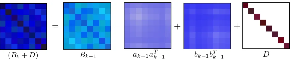
![TABLE IV[13] G. H. Golub and C. F. Van Loan,PA: Society for Industrial and Applied Mathematics (SIAM), 1996,corrected reprint of the 1983 original](https://thumb-us.123doks.com/thumbv2/123dok_us/1279409.656348/5.595.83.257.53.147/table-society-industrial-applied-mathematics-corrected-reprint-original.webp)
