97
Pervasive Attention: 2D Convolutional Neural Networks
for Sequence-to-Sequence Prediction
Maha Elbayad1,2 Laurent Besacier1 Jakob Verbeek2
Univ. Grenoble Alpes, CNRS, Grenoble INP, Inria, LIG, LJK, F-38000 Grenoble France
Abstract
Current state-of-the-art machine translation systems are based on encoder-decoder archi-tectures, that first encode the input sequence, and then generate an output sequence based on the input encoding. Both are interfaced with an attention mechanism that recombines a fixed encoding of the source tokens based on the decoder state. We propose an alterna-tive approach which instead relies on a sin-gle 2D convolutional neural network across both sequences. Each layer of our network re-codes source tokens on the basis of the out-put sequence produced so far. Attention-like properties are therefore pervasive throughout the network. Our model yields excellent re-sults, outperforming state-of-the-art encoder-decoder systems, while being conceptually simpler and having fewer parameters.
1 Introduction
Deep neural networks have made a profound im-pact on natural language processing technology in general, and machine translation in particular (Blunsom,2013;Sutskever et al.,2014;Cho et al., 2014;Jean et al.,2015;LeCun et al.,2015). Ma-chine translation (MT) can be seen as a sequence-to-sequence prediction problem, where the source and target sequences are of different and vari-able length. Current state-of-the-art approaches are based on encoder-decoder architectures ( Blun-som,2013;Sutskever et al.,2014;Cho et al.,2014; Bahdanau et al., 2015). The encoder “reads” the variable-length source sequence and maps it into a vector representation. The decoder takes this vector as input and “writes” the target sequence, updating its state each step with the most recent word that it generated. The basic encoder-decoder model is generally equipped with an attention model (Bahdanau et al.,2015), which repetitively re-accesses the source sequence during the decod-ing process. Given the current state of the decoder,
a probability distribution over the elements in the source sequence is computed, which is then used to select or aggregate features of these elements into a single “context” vector that is used by the decoder. Rather than relying on the global rep-resentation of the source sequence, the attention mechanism allows the decoder to “look back” into the source sequence and focus on salient positions. Besides this inductive bias, the attention mecha-nism bypasses the problem of vanishing gradients that most recurrent architectures encounter.
However, the current attention mechanisms have limited modeling abilities and are generally a simple weighted sum of the source representations (Bahdanau et al.,2015;Luong et al.,2015), where the weights are the result of a shallow matching between source and target elements. The atten-tion module re-combines the same source token codes and is unable to re-encode or re-interpret the source sequence while decoding.
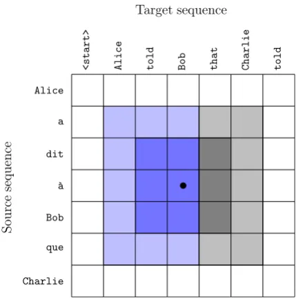
To address these limitations, we propose an al-ternative neural MT architecture, based on deep 2D convolutional neural networks (CNNs). The product space of the positions in source and tar-get sequences defines the 2D grid over which the network is defined. The convolutional filters are masked to prohibit accessing information derived from future tokens in the target sequence, obtain-ing an autoregressive model akin to generative models for images and audio waveforms (Oord et al.,2016a,b). See Figure1for an illustration.
Alice
a
dit
` a
Bob
que
Charlie
<start> Alice told Bob that Charlie told
Target sequence
Source
sequen
[image:2.595.76.291.62.279.2]ce
Figure 1: Convolutional layers in our model use masked3×3filters so that features are only com-puted from previous output symbols. Illustration of the receptive fields after one (dark blue) and two layers (light blue), together with the masked part of the field of view of a normal3×3filter (gray).
rather than using an “add-on” attention model. We validate our model with experiments on the IWSLT 2014 German-to-English (De-En) and English-to-German(En-De) tasks. We improve on state-of-the-art encoder-decoder models with at-tention, while being conceptually simpler and hav-ing fewer parameters.
In the next section we will discuss related work, before presenting our approach in detail in Sec-tion3. We present our experimental evaluation re-sults in Section4, and conclude in Section5.
2 Related work
The predominant neural architectures in machine translation are recurrent encoder-decoder net-works (Graves,2012;Sutskever et al.,2014;Cho et al., 2014). The encoder is a recurrent neu-ral network (RNN) based on gated recurrent units (Hochreiter and Schmidhuber, 1997; Cho et al., 2014) to map the input sequence into a vector rep-resentation. Often a bi-directional RNN (Schuster and Paliwal,1997) is used, which consists of two RNNs that process the input in opposite directions, and the final states of both RNNs are concatenated as the input encoding. The decoder consists of a second RNN, which takes the input encoding, and sequentially samples the output sequence one
to-ken at a time whilst updating its state.
While best known for their use in visual recog-nition models, (Oord et al.,2016a;Salimans et al., 2017; Reed et al., 2017; Oord et al., 2016c). Recent works also introduced convolutional net-works to natural language processing. The first convolutional apporaches to encoding variable-length sequences consist of stacking word vec-tors, applying 1D convolutions then aggregating with a max-pooling operator over time (Collobert and Weston,2008;Kalchbrenner et al.,2014;Kim, 2014). For sequence generation, the works of Ranzato et al. (2016); Bahdanau et al. (2017); Gehring et al. (2017a) mix a convolutional en-coder with an RNN deen-coder. The first entirely convolutional encoder-decoder models where in-troduced byKalchbrenner et al.(2016b), but they did not improve over state-of-the-art recurrent ar-chitectures. Gehring et al.(2017b) outperformed deep LSTMs for machine translation 1D CNNs with gated linear units (Meng et al., 2015; Oord et al.,2016c;Dauphin et al.,2017) in both the en-coder and deen-coder modules.
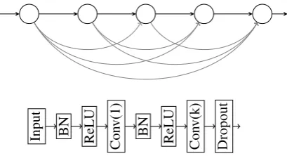
Such CNN-based models differ from their RNN-based counterparts in that temporal connec-tions are placed between layers of the network, rather than within layers. See Figure2for a con-ceptual illustration. This apparently small dif-ference in connectivity has two important conse-quences. First, it makes the field of view grow lin-early across layers in the convolutional network, while it is unbounded within layers in the recur-rent network. Second, while the activations in the RNN can only be computed in a sequential man-ner, they can be computed in parallel across the temporal dimension in the convolutional case.
condi-<start> The cat sat on the
[image:3.595.83.290.64.209.2]The cat sat on the mat
Figure 2: Illustration of decoder network topol-ogy with two hidden layers, nodes at bottom and top represent input and output respectively. Hor-izontal connections are used for RNNs, diagonal connections for convolutional networks. Vertical connections are used in both cases. Parameters are shared across time-steps (horizontally), but not across layers (vertically).
tioning on the current decoder state.
Vaswani et al.(2017) propose an architecture re-lying entirely on attention. Positional input coding together with self-attention (Parikh et al., 2016; Lin et al., 2017) replaces recurrent and convolu-tional layers.Huang et al.(2018) use an attention-like gating mechanism to alleviate an assumption of monotonic alignment in the phrase-based trans-lation model of Wang et al. (2017). Deng et al. (2018) treat the sentence alignment as a latent vari-able which they infer using a variational inference network during training to optimize a variational lower-bound on the log-likelihood.
Beyond uni-dimensional encoding/decoding. Kalchbrenner et al.(2016a) proposed a 2D LSTM model similar to our 2D CNN for machine trans-lation. Like our model, a 2D grid is defined across the input and output sequences, as in Figure 1. In their model, each cell takes input from its left and bottom neighbor. In a second LSTM stream, each cell takes input from its left and top neigh-bor, as well as from the corresponding cell in the first stream. They also observed that such a struc-ture implements an implicit form of attention, by producing an input encoding that depends on the output sequence produced so far.
Wu et al. (2017) used a CNN over the 2D source-target representation as in our work, but only as a discriminator in an adversarial training setup. They do not use masked convolutions, since
their CNN is used to predict if a given source-target pair is a human or machine translation. A standard encoder-decoder model with attention is used to generate translations.
3 Translation by 2D Convolution
In this section we present our 2D CNN translation model in detail.
Input source-target tensor. Given the source
and target pair(s,t)of lengths|s|and|t| respec-tively, we first embed the tokens in ds anddt di-mensional spaces via look-up tables. The word embeddings {x1, . . . , x|s|}and {y1, . . . , y|t|} are then concatenated to form a 3D tensor X ∈ R|t|×|s|×f0, withf0 =dt+ds, where
Xij = [yi xj]. (1)
This joint unigram encoding is the input to our convolutional network.
Convolutional layers. We use the
DenseNet (Huang et al., 2017) convolutional architecture, which is the state of the art for image classification tasks. Layers are densely connected, meaning that each layer takes as input the activations of all the preceding layers, rather than just the last one, to produce its g feature maps. The parametergis called the “growth rate” as it is the number of appended channels to the network’s output at each layer. The long-distance connections in the network improve gradient flow to early network layers during training, which is beneficial for deeper networks.
Each layer first batch-normalizes (Ioffe and Szegedy,2015) its input and apply a ReLU (Nair and Hinton, 2010) non-linearity. To reduce the computation cost, each layer first computes 4g
channels using a1×1 convolution from thef0 + (l−1)g input channels to layer l ∈ {1, . . . , L}. This is followed by a second batch-normalization and ReLU non-linearity. The second convolution has (k× dk2e) kernels, i.e. masked as illustrated in Figure 1, and generates the g output features maps to which we apply dropout (Srivastava et al., 2014). The architecture of the densely connected network is illustrated in Figure3.
Input BN ReLU
Con
v(1)
BN
ReLU Con
v(k)
[image:4.595.82.287.61.172.2]Dropout
Figure 3: Architecture of the DenseNet at block level (top), and within each block (bottom).
Target sequence prediction. Starting from the
initialf0 feature maps, each layerl ∈ {1, . . . , L}
of our DenseNet produces a tensor Hl of size
|t| × |s| ×fl, where fl is the number of output channels of that layer. To compute a distribution over the tokens in the output vocabulary, we need to collapse the second dimension of the tensor, which is given by the variable length of the input sequence, to retrieve a unique encoding for each target position.
The simplest aggregation approach is to apply max-pooling over the input sequence to obtain a tensorHpool ∈
R|t|×fL,i.e.
Hidpool= max
j∈{1,...,|s|}H
L
ijd. (2)
Alternatively, we can use average-pooling over the input sequence:
Hidpool = p1 |s|
X
j∈{1,...,|s|}
HijdL . (3)
The scaling with the inverse square-root of the source length acts as a variance stabilization term, which we find to be more effective in practice than a simple averaging.
The pooled features are then transformed to pre-dictions over the output vocabularyV, by linearly mapping them with a matrixE ∈ R|V|×fL to the vocabulary dimension |V|, and then applying a soft-max. Thus the probability distribution over
Vfor thei-th output token is obtained as
pi =SoftMax(EHipool). (4)
Alternatively, we can use E to project to dimen-sion dt, and then multiply with the target word embedding matrix used to define the input tensor. This reduces the number of parameters and gener-ally improves the performance.
Implicit sentence alignment. For a given
out-put token positioni, the max-pooling operator of Eq. (2) partitions the fL channels by assigning them across the source tokensj. Let us define
Bij ={d∈ {1, . . . , fL}|j= arg max(HijdL )}
as the channels assigned to source tokenjfor out-put token i. The energy that enters into the soft-max to predict token w ∈ V for the i-th output position is given by
eiw =
X
d∈{1,...,fL}
EwdHidpool (5)
= X
j∈{1,...,|s|}
X
d∈Bij
EwdHijdL . (6)
The total contribution of the j-th input token is thus given by
αij = X
d∈Bij
EwdHijdL , (7)
where we dropped the dependence onwfor sim-plicity. As we will show experimentally in the next section, visualizing the valuesαij for the ground-truth output tokens, we can recover an implicit sentence alignment used by the model.
Self attention. Besides pooling we can collapse
the source dimension of the feature tensor with an attention mechanism. This mechanism will gen-erate a tensorHatt that can be used instead of, or concatenated with,HPool.
We use the self-attention approach ofLin et al. (2017), which for output tokenicomputes the at-tention vectorρi∈R|s|from the activationsHiL:
ρi = SoftMax HiLw+b1|s|
, (8)
Hiatt = p|s|ρ>i HiL, (9)
wherew ∈ RfL andb ∈
Rare parameters of the
attention mechanism. Scaling of attention vectors with the square-root of the source length was also used byGehring et al.(2017b), and we found it ef-fective here as well as in the average-pooling case.
4 Experimental evaluation
4.1 Experimental setup
Data and pre-processing. We experiment with
the IWSLT 2014 bilingual dataset (Cettolo et al., 2014), which contains transcripts of TED talks aligned at sentence level, and translate between German (De) and English (En) in both directions. Following the setup of (Edunov et al., 2018), sentences longer than 175 tokens and pairs with length ratio exceeding 1.5 were removed from the original data. There are 160+7K training sentence pairs, 7K of which are separated and used for vali-dation/development. We report results on a test set of 6,578 pairs obtained by concatenating dev2010 and tst2010-2013. We tokenized and lowercased all data using the standard scripts from the Moses toolkit (Koehn et al.,2007).
For open-vocabulary translation, we segment sequences using joint byte pair encoding ( Sen-nrich et al.,2016) with 14K merge operations on the concatenation of source and target languages. This results in a German and English vocabularies of around 12K and 9K types respectively.
Implementation details. Unless stated
other-wise, we use DenseNets with masked convolu-tional filters of size 5×3, as given by the light blue area in Figure 1. To train our models, we use maximum likelihood estimation (MLE) with Adam(β1 = 0.9, β2 = 0.999, = 1e−8)starting
with a learning rate of5e−4that we scale by a fac-tor of 0.8 if no improvement (δ≤0.01) is noticed on the validation loss after three evaluations, we evaluate every 8K updates.
After training all models up to 40 epochs, the best performing model on the validation set is used for decoding the test set. We use a beam-search of width 5 without any length or coverage penalty and measure translation quality using the BLEU metric (Papineni et al.,2002).
Baselines. For comparison with
state-of-the-art architectures, we implemented a bidirec-tional LSTM encoder-decoder model with dot-product attention (Bahdanau et al., 2015; Luong et al.,2015) using PyTorch (Paszke et al.,2017), and used Facebook AI Research Sequence-to-Sequence Toolkit (Gehring et al., 2017b) to train the ConvS2S and Transformer (Vaswani et al., 2017) models on our data.
For the Bi-LSTM encoder-decoder, the encoder is a single layer bidirectional LSTM with input embeddings of size 128 and a hidden state of size
Model BLEU Flops×105 #params
Average 31.57±0.11 3.63 7.18M Max 33.70±0.06 3.44 7.18M Attn 32.07±0.13 3.61 7.24M Max, gated 33.66±0.16 3.49 9.64M [Max, Attn] 33.81±0.03 3.51 7.24M
Table 1: Our model (L= 24, g= 32, ds=dt= 128) with different pooling operators and using gated convolutional units.
256 (128 in each direction). The decoder is a sin-gle layer LSTM with similar input size and a hid-den size of 256, the target input embeddings are also used in the pre-softmax projection. For regu-larization, we apply a dropout of rate 0.2 to the in-puts of both encoder and decoder and to the output of the decoder prior to softmax. As in (Bahdanau et al.,2015), we refer to this model as RNNsearch. The ConvS2S model we trained has embed-dings of dimension 256, a 16-layers encoder and 12-layers decoder. Each convolution uses3×1 fil-ters and is followed by a gated linear unit with a total of 2×256channels. Residual connections link the input of a convolutional block to its out-put. We first trained the default architecture for this dataset as suggested in FairSeq (Gehring et al., 2017b), which has only 4 layers in the encoder and 3 in the decoder, but achieved better results with the deeper version described above. The model is trained with MLE using Nesterov accelerated gradient with a momentum of 0.99 and an initial learning rate of 0.25 decaying by a factor of 0.1 every epoch. ConvS2S is also regularized with a dropout rate of 0.2.
For the transformer model, use the settings of (Vaswani et al.,2017). We use token embeddings of dimension 512, and the encoder and decoder have 6 layers and 8 attention heads. For the in-ner layer in the per-position feed-forawrd network we use df f = 2048. For MLE training we use Adam(β1 = 0.9, β2 = 0.98, = 1e−8)(Kingma
and Ba, 2015), and a learning rate starting from
1e−5that is increased during 4,000 warm-up steps then used a learning rate of 5e−4 that follows an inverse-square-root schedule afterwards (Vaswani et al.,2017). Similar to previous models we set the dropout rate to 0.2.
4.2 Experimental results
Architecture evaluation. In this section we
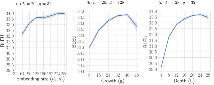
(a)L= 20, g= 32 (b)L= 20, d= 128 (c)d= 128, g= 32
Figure 4: Impact of token embedding size, number of layers (L), and growth rate (g).
model: the token embedding dimension, depth, growth rate and filter sizes. We also evaluate dif-ferent aggregation mechanisms across the source dimension: max-pooling, average-pooling, and at-tention.
In each chosen setting, we train five models with different initializations and report the mean and standard deviation of the BLEU scores. We also state the number of parameters of each model and the computational cost of training, estimated in a similar way asVaswani et al.(2017), based on the wall clock time of training and the GPU single precision specs.
In Table 1 we see that using max-pooling in-stead average-pooling across the source dimen-sion increases the performance with around 2 BLEU points. Scaling the average representa-tion withp|s|Eq. (3) helped improving the per-formance but it is still largely outperformed by the max-pooling. Adding gated linear units on top of each convolutional layer does not improve the BLEU scores, but increases the variance due to the additional parameters. Stand-alone self-attentioni.e. weighted average-pooling is slightly better than uniform average-pooling but it is still outperformed by max-pooling. Concatenating the max-pooled features (Eq. (2)) with the represen-tation obtained with self-attention (Eq. (9)) leads to a small but significant increase in performance, from 33.70 to 33.81. In the remainder of our ex-periments we only use max-pooling for simplicity, unless stated otherwise.
In Figure 4we consider the effect of the token embedding size, the growth rate of the network, and its depth. The token embedding size together
with the growth rategcontrol the number of fea-tures that are passed though the pooling operator along the source dimension, and that can be used used for token prediction. Using the same embed-ding sized= dt =dson both source and target, the total number of features for token prediction produced by the network is fL = 2d+gL. In Figure 4 we see that for token embedding sizes between 128 to 256 lead to BLEU scores vary between 33.5 and 34. Smaller embedding sizes quickly degrade the performance to 32.2 for em-beddings of size 64. The growth rate (g) has an im-portant impact on performance, increasing it from 8 to 32 increases the BLEU scrore by more than 2.5 point. Beyondg = 32performance saturates and we observe only a small improvement. For a good trade-off between performance and compu-tational cost we chooseg = 32for the remaining experiments. The depth of the network also has an important impact on performance, increasing the BLEU score by about 2 points when increasing the depth from 8 to 24 layers. Beyond this point per-formance drops due to over-fitting, which means we should either increase the dropout rate or add another level of regularization before considering deeper networks. The receptive field of our model is controlled by its depth and the filter size. In Ta-ble 2, we note that narrower receptive fields are better than larger ones with less layers at equiva-lent complextitiese.g. comparing (k= 3, L= 20) to (k = 5, L = 12), and (k = 5, L = 16) with (k= 7, L= 12).
Comparison to the state of the art. We
Ta-k L BLEU Flops×105 #params
3 16 32.99±0.08 2.47 4.32M 3 20 33.18±0.19 3.03 4.92M
5 8 31.79±0.09 0.63 3.88M 5 12 32.87±0.07 2.61 4.59M 5 16 33.34±0.12 3.55 5.37M 5 20 33.62±0.07 3.01 6.23M 5 24 33.70±0.06 3.44 7.18M 5 28 33.46±0.23 5.35 8.21M
[image:7.595.311.524.60.233.2]7 12 32.58±0.12 2.76 5.76M
Table 2: Performance of our model (g= 32, ds=
dt= 128) for different filter sizeskand depthsL and filter sizesk.
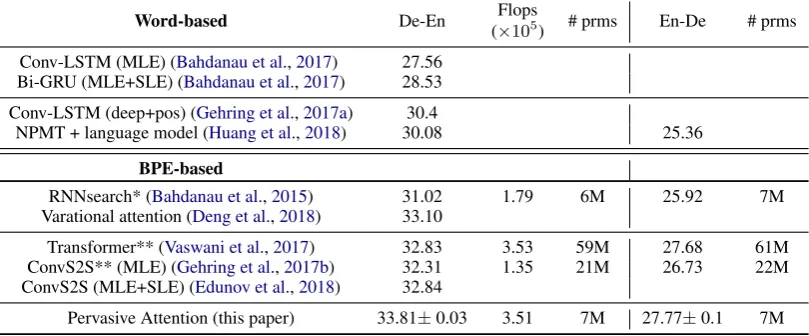
ble3for both directions German-English (De-En) and English-German (En-De). We refer to our model as Pervasive Attention . Unless stated oth-erwise, the parameters of all models are trained using maximum likelihood estimation (MLE). For some models we additionally report results ob-tained with sequence level estimation (SLE, e.g. using reinforcement learning approaches), typi-cally aiming directly to optimize the BLEU mea-sure rather than the likelihood of correct transla-tion.
First of all we find that all results obtained using byte-pair encodings (BPE) are superior to word-based results. Our model has about the same num-ber of parameters as RNNsearch, yet improves performance by almost 3 BLEU points. It is also better than the recent work of Deng et al.(2018) on recurrent architectures with variational atten-tion. Our model outperforms both the recent trans-former approach ofVaswani et al.(2017) and the convolutional model of Gehring et al.(2017b) in both translation directions, while having about 3 to 8 times fewer parameters. Our model has an equivalent training cost to the transformer (as im-plemented in fairseq) while the convs2s imple-mentation is well optimized with fast running 1d-convolutions leading to shorter training times.
Performance across sequence lengths. In
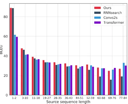
Fig-ure 5 we consider translation quality as a func-tion of sentence length, and compare our model to RNNsearch, ConvS2S and Transformer. Our model gives the best results across all sen-tence lengths, except for the longest ones where ConvS2S and Transformer are better. Overall, our model combines the strong performance of RNNsearch on short sentences with good
perfor-Figure 5: BLEU scores across sentence lengths.
mance of ConvS2S and Transformer on longer ones.
Implicit sentence alignments. Following the
method described in Section3, we illustrate in Fig-ure 6 the implicit sentence alignments the max-pooling operator produces in our model. For ref-erence we also show the alignment produced by our model using self-attention. We see that with both max-pooling and attention qualitatively sim-ilar implicit sentence alignments emerge.
Notice in the first example how the max-pool model, when writingI’ve been working, looks at arbeite but also at seit which indicates the past tense of the former. Also notice some cases of non-monotonic alignment. In the first examplefor some time occurs at the end of the English sen-tence, but seit einiger zeit appears earlier in the German source. For the second example there is non-monotonic alignment around the negation at the start of the sentence. The first example illustrates the ability of the model to translate proper names by breaking them down into BPE units. In the second example the German word Karriereweg is broken into the four BPE units karri,er,e,weg. The first and the fourth are mainly used to produce the English a carreer, while for the subsequentpaththe model looks atweg.
[image:7.595.86.278.63.187.2](a) Max-pooling (b) Self-attention
(c) Max-pooling (d) Self-attention
[image:8.595.72.531.81.681.2](e) Max-pooling (f) Self-attention
Word-based De-En Flops
(×105) # prms En-De # prms
Conv-LSTM (MLE) (Bahdanau et al.,2017) 27.56 Bi-GRU (MLE+SLE) (Bahdanau et al.,2017) 28.53
Conv-LSTM (deep+pos) (Gehring et al.,2017a) 30.4
NPMT + language model (Huang et al.,2018) 30.08 25.36
BPE-based
RNNsearch* (Bahdanau et al.,2015) 31.02 1.79 6M 25.92 7M Varational attention (Deng et al.,2018) 33.10
Transformer** (Vaswani et al.,2017) 32.83 3.53 59M 27.68 61M ConvS2S** (MLE) (Gehring et al.,2017b) 32.31 1.35 21M 26.73 22M ConvS2S (MLE+SLE) (Edunov et al.,2018) 32.84
[image:9.595.96.501.66.234.2]Pervasive Attention (this paper) 33.81±0.03 3.51 7M 27.77±0.1 7M
Table 3: Comparison to state-of-the art results on IWSLT German-English translation. (*): results ob-tained using our implementation. (**): results obob-tained using FairSeq (Gehring et al.,2017b).
phrase, and progressively from the part of the source phrase that remains to be decoded.
5 Conclusion
We presented a novel neural machine translation architecture that departs from the encoder-decoder paradigm. Our model jointly encodes the source and target sequence into a deep feature hierarchy in which the source tokens are embedded in the context of a partial target sequence. Max-pooling over this joint-encoding along the source dimen-sion is used to map the features to a prediction for the next target token. The model is implemented as 2D CNN based on DenseNet, with masked con-volutions to ensure a proper autoregressive factor-ization of the conditional probabilities.
Since each layer of our model re-encodes the input tokens in the context of the target sequence generated so far, the model has attention-like prop-erties in every layer of the network by construc-tion. Adding an explicit self-attention module therefore has a very limited, but positive, effect. Nevertheless, the max-pooling operator in our model generates implicit sentence alignments that are qualitatively similar to the ones generated by attention mechanisms. We evaluate our model on the IWSLT’14 dataset, translation German to En-glish and vice-versa. We obtain excellent BLEU scores that compare favorably with the state of the art, while using a conceptually simpler model with fewer parameters.
We hope that our alternative joint source-target encoding sparks interest in other alternatives to the encoder-decoder model. In the future, we plan to
explore hybrid approaches in which the input to our joint encoding model is not provided by token-embedding vectors, but the output of 1D source and target embedding networks,e.g. (bi-)LSTM or 1D convolutional. We also want to explore how our model can be used to translate across multiple language pairs.
Our PyTorch-based implementation is
avail-able at https://github.com/elbayadm/
attn2d.
References
D. Bahdanau, P. Brakel, K. Xu, A. Goyal, R. Lowe, J. Pineau, A. Courville, and Y. Bengio. 2017. An actor-critic algorithm for sequence prediction. In
ICLR.
D. Bahdanau, K. Cho, and Y. Bengio. 2015. Neural machine translation by jointly learning to align and translate. InICLR.
N. Kalchbrenner P. Blunsom. 2013. Recurrent contin-uous translation models. InACL.
M. Cettolo, J. Niehues, S. Stüker, L. Bentivogli, and M. Federico. 2014. Report on the 11th IWSLT eval-uation campaign. InIWSLT.
K. Cho, B. van Merrienboer, Ç. Gülçehre, D. Bah-danau, F. Bougares, H. Schwenk, and Y. Bengio. 2014. Learning phrase representations using RNN encoder-decoder for statistical machine translation. InEMNLP.
Y. Dauphin, A. Fan, M. Auli, and D. Grangier. 2017. Language modeling with gated convolutional net-works. InICML.
Y. Deng, Y. Kim, J. Chiu, D. Guo, and A. Rush. 2018. Latent alignment and variational attention. arXiv preprint arXiv:1807.03756.
S. Edunov, M. Ott, M. Auli, D. Grangier, and M. Ran-zato. 2018. Classical structured prediction losses for sequence to sequence learning. InNAACL.
J. Gehring, M. Auli, D. Grangier, and Y. Dauphin. 2017a. A convolutional encoder model for neural machine translation. InACL.
J. Gehring, M. Auli, D. Grangier, D. Yarats, and Y. Dauphin. 2017b. Convolutional sequence to se-quence learning. InICML.
A. Graves. 2012. Sequence transduction with recurrent neural networks. arXiv preprint arXiv:1211.3711.
S. Hochreiter and J. Schmidhuber. 1997. Long short-term memory. Neural Computation, 9(8):1735– 1780.
G. Huang, Z. Liu, L. van der Maaten, and K. Wein-berger. 2017. Densely connected convolutional net-works. InCVPR.
P. Huang, C. Wang, S. Huang, D. Zhou, and L. Deng. 2018. Towards neural phrase-based machine trans-lation. InICLR.
S. Ioffe and C. Szegedy. 2015. Batch normalization: Accelerating deep network training by reducing in-ternal covariate shift. InICML.
S. Jean, K. Cho, R. Memisevic, and Y. Bengio. 2015. On using very large target vocabulary for neural ma-chine translation. InACL.
N. Kalchbrenner, I. Danihelka, and A. Graves. 2016a. Grid long short-term memory. InICLR.
N. Kalchbrenner, L. Espeholt, K. Simonyan, A. van den Oord, A. Graves, and K. Kavukcuoglu. 2016b. Neural machine translation in linear time. arXiv, arXiv:1610.10099.
N. Kalchbrenner, E. Grefenstette, and P. Blunsom. 2014. A convolutional neural network for modelling sentences. InACL.
Y. Kim. 2014. Convolutional neural networks for sen-tence classification. InACL.
D. Kingma and J. Ba. 2015. Adam: A method for stochastic optimization. InICLR.
P. Koehn, H. Hoang, A. Birch, C. Callison-Burch, M. Federico, N. Bertoldi, B. Cowan, W. Shen, C. Moran, R. Zens, C. Dyer, O. Bojar, A. Constantin, and E. Herbst. 2007. Moses: Open source toolkit for statistical machine translation. InACL.
Y. LeCun, Y. Bengio, and G. Hinton. 2015. Deep learn-ing.Nature, 52:436–444.
Z. Lin, M. Feng, C. dos Santos, M. Yu, B. Xiang, B. Zhou, and Y. Bengio. 2017. A structured self-attentive sentence embedding. InICLR.
T. Luong, H. Pham, and C. Manning. 2015. Effective approaches to attention-based neural machine trans-lation. InEMNLP.
F. Meng, Z. Lu, M. Wang, H. Li, W. Jiang, and Q. Liu. 2015. Encoding source language with convolutional neural network for machine translation. InACL.
V. Nair and G. Hinton. 2010. Rectified linear units im-prove restricted Boltzmann machines. InICML.
A. van den Oord, S. Dieleman, H. Zen, K. Simonyan, O. Vinyals, A. Graves, N. Kalchbrenner, A. Senior, and K. Kavukcuoglu. 2016a. Wavenet: a genera-tive model for raw audio. InISCA Speech Syntesis Workshop.
A. van den Oord, N. Kalchbrenner, and K. Kavukcuoglu. 2016b. Pixel recurrent neu-ral networks. InICML.
A. van den Oord, N. Kalchbrenner, O. Vinyals, L. Espe-holt, A. Graves, and K. Kavukcuoglu. 2016c. Con-ditional image generation with PixelCNN decoders. InNIPS.
K. Papineni, S. Roukos, T. Ward, and W.-J. Zhu. 2002. BLEU: a method for automatic evaluation of ma-chine translation. InACL.
A. Parikh, O. Täckström, D. Das, and J. Uszkoreit. 2016. A decomposable attention model for natural language inference. InEMNLP.
A. Paszke, S. Gross, S. Chintala, G. Chanan, E. Yang, Z. DeVito, Z. Lin, A. Desmaison L. Antiga, and A. Lerer. 2017. Automatic differentiation in py-torch. InNIPS-W.
M. Ranzato, S. Chopra, M. Auli, and W. Zaremba. 2016. Sequence level training with recurrent neural networks. InICLR.
S. Reed, A. van den Oord, N. Kalchbrenner, S. Gómez Colmenarejo, Z. Wang, D. Belov, and N. de Freitas. 2017. Parallel multiscale autoregressive density es-timation. InICML.
T. Salimans, A. Karpathy, X. Chen, and D. Kingma. 2017. PixelCNN++: Improving the PixelCNN with discretized logistic mixture likelihood and other modifications. InICLR.
M. Schuster and K. Paliwal. 1997. Bidirectional recurrent neural networks. Signal Processing, 45(11):2673–2681.
N. Srivastava, G. Hinton, A. Krizhevsky, I. Sutskever, and R. Salakhutdinov. 2014. Dropout: A simple way to prevent neural networks from overfitting.
JMLR.
I. Sutskever, O. Vinyals, and Q. Le. 2014. Sequence to sequence learning with neural networks. InNIPS.
A. Vaswani, N. Shazeer, N. Parmar, J. Uszkoreit, L. Jones, A. Gomez, L. Kaiser, and I. Polosukhin. 2017. Attention is all you need. InNIPS.
C. Wang, Y. Wang, P.-S. Huang, A. Mohamed, D. Zhou, and L. Deng. 2017. Sequence modeling via segmentations. InICML.
L. Wu, Y. Xia, L. Zhao, F. Tian, T. Qin, J. Lai, and T.-Y. Liu. 2017. Adversarial neural machine translation.
arXiv, arXiv:1704.06933.