Reference Crop Evapotranspiration spatially interpolated and temporally distributed in Java

“Reference Crop Evapotranspiration spatially

interpolated and temporally distributed in Java”

Bachelor Thesis

April – July 2009

Author: Erik Ensing

Student number: s0138843

Supervisors:

1

Summary

As the water scarcity in the agricultural sector increases, there is a greater demand for more efficient irrigation. With better predictions of the reference crop evapotranspiration ( ), more efficient irrigation scheduling can be done. The is the evapotranspiration rate from a reference surface, which resembles a uniform surface of green grass with adequate water. In this study a model has been made for determining the on Java. This model can calculate the interpolated at a certain location when the coordinates and the predicted wind speed at that location are given. These calculations can be carried out for each month and the average over the year. The grid size of the interpolation is 1 by 1 minute, which is about 1.84 by 1.84 kilometers.

For this study, data from 24 measurement stations on Java have been used. For 20 of these stations, the data has been supplied by the Food and Agriculture Organization of the United Nations (FAO). For the remaining 4 stations, the data has been supplied by the Indonesian National Agency for Meteorology, Climatology and Geophysics (BMKG). Also, altitude data from GEBCO has been used.

In this research, five methods have been used for predicting the . In each of these methods the is interpolated. Method 1 consists of interpolating the values calculated with data from the measurement stations, using triangle-based interpolation methods. In Method 2 the is divided into an aerodynamic and a radiation component, which are individually interpolated. In this method, the wind speed is partially excluded from these components, which means the given or predicted wind speed is used to calculate the . In Methods 3, 4 and 5 the is divided into four components representing the aerodynamic part, the radiation part, the psychometric constant and the saturation vapor pressure relationship. Here the wind speed is entirely excluded from these components. In Method 3 the psychometric constant is interpolated, in Method 4 it is calculated using the altitude data from GEBCO and in Method 5 it is calculated using the altitude given in the data from the measurement stations.

Method 1 had better results than Method 2, meaning plain interpolation is better than dividing the into two components and using the given or predicted wind speed. Methods 3, 4 and 5 all had better results than Method 1. Method 4 had worse results than Method 3, but better results than Method 5. Methods 4 and 5 both had worse results than Method 3, because the reduction of the error in the psychometric constant increased the overall error.

In a following research, Method 4 or 5 should be improved, because for those methods the sum of absolute errors of the components is lower.

The results showed that the model currently does not give good predictions for locations with high altitude differences with respect to their neighboring measurement locations. This is probably because the model does not yet take into account the temperature decrease at higher altitudes, this can be done in a future study. When the temperature is interpolated in a better way, the errors in all components except for the psychometric constant could decrease. Currently errors in these components cause most of the errors in the , so interpolating the temperature in a better way can greatly improve the model.

2

Preface

I started with the preparation for my research and visit in Indonesia in the beginning of February this year. I did research on a model for predicting evapotranspiration in Java. The research was done in Bandung, at a rather quickly growing company called LabMath. I did research on the model for about three months there. There were some complications and I was ill in the first few weeks, but I think I managed to do the research quite well. The complications I speak of include a change of supervisor in Indonesia – because my first supervisor quit the company – and not being able to obtain more data in time. However, I think the model has developed quite well during the course of my research. While improvements can certainly be made, I am pleased with what the model can do now.

I think I learned a lot during my stay in Indonesia. Not only from doing my research, but also from living there. The culture and living circumstances in Indonesia are a lot different from those in Europe. There is a very big difference between rich and poor in Indonesia, the safety measures are rather poor and there is a lot of chaos. Because of my research I learned to work a lot better with MatLab, which will probably be very useful for my study and work in the future. I also learned that it is very hard to obtain reliable data in Indonesia.

I would like to give my thanks to a number of people who helped me during this research.

To start with, I would like to thank my supervisors Martijn Booij, “Dody” Satyanto Krido Saptomo and Brenny van Groesen for their good advice and support.

I would also like to thank all the students and staff at LabMath, for their help and friendliness. You were all good friends to me. A lot of you taught Ferdinand and me how to get around town and some of you even took us on very nice trips. Because of this, the office felt like a very warm place to me.

Next, I would like to thank Ferdinand. He also did his internship at LabMath and we stayed at the same student housing. He was really helpful and a good companion. I had a lot of fun with him in the weekends.

3

Table of Contents

Summary ... 1

Preface ... 2

1. Introduction ... 4

1.1. Problem context ... 4

1.2. Objective and research questions ... 4

1.3. Outline ... 5

2. Calculation of the reference crop evapotranspiration ... 6

2.1. Deriving the FAO-56 Penman-Monteith equation ... 6

2.2. Calculation of the variables in the FAO-56 Penman-Monteith equation ... 8

2.3. FAO-56 Penman-Monteith variables and parameters ... 11

2.3.1. Parameters used in the model ... 12

2.3.2. Variables used as model input ... 12

3. Study area and data ... 13

3.1. Study area and measurement locations... 13

3.2. Meteorological data ... 13

3.3. Elevation data ... 15

4. Modeling and interpolation methods ... 17

4.1. Interpolation methods in MatLab ... 17

4.2. Modeling methods ... 18

4.2.1. Method 1: Interpolating the ETo ... 18

4.2.2. Method 2: The α and β method ... 18

4.2.3. Method 3: The abcd method ... 19

4.2.4. Method 4: The abcd method, but using altitude data for determining γ ... 19

4.2.5. Method 5: The abcd method, but using the given height to determine γ ... 20

5. Results and discussion ... 21

5.1. Results ... 21

5.1.1. Monthly errors ... 21

5.1.2. Errors per station ... 24

5.1.3. Average errors per method ... 27

5.1.4. Monthly variations ... 28

5.2. Discussion ... 31

6. Conclusions and recommendations ... 33

6.1. Conclusions ... 33

6.2. Recommendations... 34

References ... 35

Appendices ... 36

Appendix I: List of symbols ... 36

Appendix II: MatLab Model ... 38

Appendix III: Code of the MatLab m-files ... 48

4

1.

Introduction

1.1.

Problem context

The global climate conditions keep changing. These changes directly affect the water cycle and thus the individual components of the water balance. Due to this, Java faces various severe problems with water. Rivers are flooding in many areas, which causes great human, social and economic problems during the wet season. In the dry season and at several times in the wet season there is a severe shortage of water for human consumption, industrial use, agricultural use and natural vegetation. The dry season is taking longer, while the wet season is shorter with heavier rainfall intensity (Case, Ardiansyah, & Spector, 2007). According to the IPCC (2007), the condition will get even worse in the future. The freshwater availability is projected to decrease, more floods are projected and more droughts are expected in Southeast Asia.

Because of these changes, farmers more often face severe water shortages. This means they need to be very efficient with their irrigation water. For the calculation of the amount of efficient irrigation water in agriculture, evapotranspiration (ET) is an important factor, because ET is a source of irrigation water loss. A lot of water is used for the production of rice and cassava (Bulsink, 2008). However, there is no model that can easily predict the ET over all of Java for a few days ahead yet. This means farmers are often uncertain if they need to use irrigation water or not, while not much fresh water is available for irrigation (Safrina, 2009).

Also the type of crops is of great influence to the ET, because every crop has a different Leaf Area Index (LAI) and a different aerodynamic resistance. The aerodynamic resistance determines the transfer of heat and water vapor from the evaporating surface into the air and the LAI is determined by dividing the upper leaf surface by the surface area of the land beneath the vegetation. Deforestation will result in changes of energy and water budgets of land surface, which will cause local and regional environmental condition changes as the consequence. As shown by Olchev et. al. (2008), a deforestation of around 15% for agricultural and urban activities in Central Sulawesi will considerably increase ground evaporation by 21%. Uncontrolled urbanization causes an increase in overland run-off and river discharge which often results in flooding and landslides. Uncontrolled urbanization reduces the ground water, which is used by the agricultural sector. When the ground water level decreases, less water becomes available for direct human consumption and the environment.

There is a high uncertainty in what is going to happen in certain local or regional areas when the climate changes. A sensitive spatial averaging method is needed in view of the large spatial variability of the ET. When the climate changes, farmers cannot rely on their experience with the weather. A model is needed so that people can make well informed choices. This model needs to show farmers when they should use irrigation and what the effect of using other types of crops is. The model that has been developed in this study does not take into account the crop types at various locations. The ET for a specific reference crop is given instead, which can be converted into the ET for a specific crop type, by multiplying it with a crop dependent coefficient. What is important for this model is that it is not too complicated, but it should still give reliable results. In this research will be checked if an easy and reliable model can be made for predicting the ET, which uses the predicted wind speed as input. This is because a preliminary study showed that the spatial and seasonal variations of the ET are very dependent on the wind speed and less dependent on the temperature in Java (Widarta, 2009).

1.2.

Objective and research questions

The goal of this research is formulated as follows:

5 From the research objective, the following research questions were derived:

1. What are the relevant weather parameters which can be used as input for the model? 1.1. Which data are needed?

1.2. Which data are available? 1.3. Are the available data reliable?

2. How do these relevant weather parameters relate to the reference crop evapotranspiration? 2.1. Which equations are used to calculate potential evapotranspiration?

2.2. How are these equations used in the (different versions of) the model?

2.3. Which assumptions are made and what values are chosen for the different parameters? 3. Which spatial inter- and extrapolation methods should be used in the modeling of the reference

crop evapotranspiration?

3.1. Which interpolation methods are available and what are their pros and cons?

3.2. Which spatial characteristics should the spatial inter- and extrapolation method be based on?

1.3.

Outline

In chapter 2 the various equations for calculating the reference crop evapotranspiration are shown. In particular, the FAO-56 Penman-Monteith equation and the calculation of the variables in this equation will be considered. Also an overview is given of the different variables and parameters used in the model. The values that are chosen for the different parameters are shown and the variables used as input for the model are shown.

In chapter 3 the study area, the measurement locations and the measurement data are discussed. Meteorological data from 24 stations on Java have been used, the locations of the stations are shown and the source of the data is discussed. Also the elevation data from GEBCO that is used in Method 4 of this model is discussed.

In chapter 4 the different modeling and interpolation methods are explained. In total 5 methods have been used in this research. Explained is how the predicted reference crop evapotranspiration is determined in each of these methods.

In chapter 5 the results of the different modeling methods and interpolation methods are shown. Also, the phenomena seen in the results and the limitations of this study will be discussed in this chapter.

In the final chapter, chapter 6, the conclusions of this research and recommendations for a possible following research are given.

6

2.

Calculation of the reference crop evapotranspiration

2.1.

Deriving the FAO-56 Penman-Monteith equation

In the model that has been developed in this study, the reference crop evapotranspiration ( ) is calculated. For calculating this, the guidelines for computing crop water requirements from the FAO (Allen et. al., 1998) are used. All equations shown in this chapter are taken from these guidelines. A list of all symbols used in these equations can be found in Appendix I. The FAO derived a standard formula for the from the original Monteith evapotranspiration equation. The Penman-Monteith equation is as follows:

(eq. 2.1)

Where:

: latent heat flux (representing the evapotranspiration) [MJ m-2 day-1]

: slope of the relationship between the saturation vapor pressure and temperature [kPa °C-1] : net radiation [MJ m-2 day-1]

: soil heat flux density [MJ m-2 day-1]

: mean air density at constant pressure [kg m-3] : specific heat at constant pressure [MJ kg-1 °C-1] : saturation vapor pressure [kPa]

: actual vapor pressure [kPa]

: saturation vapor pressure deficit [kPa] : psychometric constant [kPa °C-1]

: (bulk) surface resistance [s m-1] : aerodynamic resistance [s m-1]

The reference crop evapotranspiration is the evapotranspiration rate from a reference surface. It is assumed that there is sufficient water at the reference surface. The reference surface is assumed to have crops with the following characteristics:

"A hypothetical reference crop with an assumed crop height of 0.12 m, a fixed surface resistance of 70 s m-1and an albedo of 0.23."

This means that the reference surface closely resembles an extensive surface of green grass of uniform height, actively growing, completely shading the ground and with adequate water.

As a result of the assumptions in the definition of the reference surface, a part of the Penman-Monteith equation can be evaluated. From the definition, the following is known:

(surface resistance) (crop height)

(albedo or canopy reflection coefficient)

Using the crop height, the aerodynamic resistance can be calculated. The aerodynamic resistance ( ) is calculated using the following equation:

(eq. 2.2)

Where:

7 : roughness length governing momentum transfer [m]

: roughness length governing transfer of heat and vapour [m] : von Karman’s constant, 0.41 *-]

: wind speed at height z [m s-1]

The zero plane displacement height, the roughness length governing momentum transfer and the roughness length governing transfer of heat and vapor are calculated using the following equations:

With h = 0.12 and all measurements taken at 2 m height, the aerodynamic resistance of the reference surface becomes:

(eq. 2.3)

Also, the “ ”-fraction in the Penman-Monteith equation can be written differently. The values for and are calculated with the following equations:

(eq. 2.4)

Where:

: atmospheric pressure [kPa]

: the mean of the monthly averaged maximum and minimum temperatures (measured at 2m height) [°C]

: specific gas constant, 0.287 [kJ kg-1 K-1]

(eq. 2.5)

Where:

: ratio molecular weight of water vapour/dry air, 0.622 [-] : latent heat of vaporization, 2.45 [MJ kg-1]

So the equation for the “ ”-fraction becomes:

(eq. 2.6)

When this is multiplied by 86400 to calculate the per day and divided by 2.45 to transfer from [MJ °C-1 day-1 m-2] to [mm °C-1 day-1], the fraction becomes:

(eq. 2.7)

Also, a transfer factor is needed for the radiation part of the Penman-Monteith equation, to convert this from [MJ m-2 day-1] to [mm day-1]. This transfer factor is 0.408.

8 So the FAO-56 Penman-Monteith equation becomes:

(eq. 2.8)

Where:

: reference evapotranspiration [mm day-1] : wind speed at 2 m height [m s-1]

2.2.

Calculation of the variables in the FAO-56 Penman-Monteith equation

Slope of saturation vapour pressure curve (Δ)

(eq. 2.9)

Net radiation at the crop surface (Rn)

(eq. 2.10)

Where:

: net solar or shortwave radiation [MJ m-2 _day-1_]

: net outgoing longwave radiation [MJ m-2 day-1]

(eq. 2.11)

Where:

: albedo or canopy reflection coefficient, 0.23 for the reference surface [-] : incoming solar or shortwave radiation [MJ m-2 day-1]

(eq. 2.12)

Where:

: Stefan-Boltzmann constant, 4.903 · 10-9 [MJ K-4 m-2 day-1] : maximum absolute temperature during the 24-hour period [K] : minimum absolute temperature during the 24-hour period [K] : relative shortwave radiation (limited to ≤ 1.0) [-]

9 (eq. 2.13)

Where:

: actual duration of sunshine [hour] : daylight hours [hour]

: relative sunshine duration [-]

: extraterrestrial radiation [MJ m-2 day-1]

: regression constant, expressing the fraction of extraterrestrial radiation reaching the earth on overcast days (n = 0)

: additional regression constant, expressing the extra fraction of extraterrestrial radiation reaching the earth during sunshine hours

: fraction of extraterrestrial radiation reaching the earth on clear days (n = N)

(eq. 2.14)

(eq. 2.15)

Where:

: sunset hour angle [rad]

(eq. 2.16)

Where:

: latitude [rad]

: solar decimation [rad]

(eq. 2.17)

Where:

: solar constant, 0.0820 [MJ m-2 min-1] : inverse relative distance Earth-Sun

(eq. 2.18)

Where:

: number of the day in the year from 1 (1 January) to 365 or 366 (31 December)

(eq. 2.19)

(eq. 2.20)

Where:

10

Soil heat flux density (G)

When assuming a constant soil heat capacity of 2.1 MJ m-3 °C-1 and an appropriate soil depth, equation 2.21 can be derived for G for monthly periods. These assumptions may be very rough, but the soil heat flux is very small compared to (and as seen in equation 2.8 it is subtracted from that) and can often even be ignored, so the rough assumptions only cause very small errors.

(eq. 2.21)

Where:

: soil heat flux density in month i [MJ m-2 day-1]

: the mean of the monthly averaged maximum and minimum temperatures in the next month (measured at 2m height) [°C]

: the mean of the monthly averaged maximum and minimum temperatures in the previous month (measured at 2m height) [°C]

Psychometric constant (γ)

(eq. 2.22)

(eq. 2.23)

Where:

: elevation above sea level [m]

Saturation vapor pressure (es) and actual vapor pressure (ea)

(eq. 2.24)

Where:

: saturation vapour pressure at the air temperature [kPa]

: mean of the daily maximum temperatures taken over the month [°C] : mean of the daily minimum temperatures taken over the month [°C]

(eq. 2.25)

Where:

: the mean relative humidity [-]

This is a less desirable equation for calculating the actual vapor pressure, but psychometric data was not available and only the mean relative humidity is given.

(eq. 2.26)

Where:

11

2.3.

FAO-56 Penman-Monteith variables and parameters

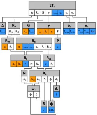
In the following schedule a very basic overview is given of the relation between the parameters and variables in the calculation of the reference crop evapotranspiration. In this model, parameters are constants, which means they have only one value in the entire model. Variables on the other hand, have different values depending on the time and/or location of the measurements they relate to. In this schedule, the blue blocks stand for variables and the orange blocks stand for parameters. Under each gray block are blocks with therein the input needed to calculate the value of the quantity the gray block represents.

ET

Δ Rn G γ es ea

Δ

Tmean

R

Rns Rnl

R

α Rs

R

σ Tmax,KTmin,K ea Rs Rso

G

cs

R

as bs n N Ra

N

ωs

ω

δ φ

R

z Ra

R

Gsc δ φ dr

P

γ

cp λ ε P

z

e

TmaxTmin

e

Tmin RH

δ

J

φ

Lat.

d

J u2

ωs

Tmax Tmean

Tmean

Figure 2.1: Schedule of the variables and parameters in the model.

12

2.3.1. Parameters used in the model

As can be seen in the schedule above, the parameters used in the model are the following:

= 1.013 · 10-3 [MJ kg-1 °C-1], specific heat at constant pressure = 2.45 [MJ kg-1], latent heat of vaporization

= 0.622 [-], ratio molecular weight of water vapor/dry air = 0.23 [-], albedo or canopy reflection coefficient

= 4.903 · 10-9 _{[MJ K}-4 _m-2 _day-1_{], Stefan-Boltzmann constant}

= 0.25 [-], regression constant, expressing the fraction of extraterrestrial radiation reaching the earth on overcast days (n = 0)

= 0.50 [-], additional regression constant, expressing the extra fraction of extraterrestrial radiation reaching the earth during sunshine hours

= 0.75 [-], fraction of extraterrestrial radiation reaching the earth on clear days (n = N) = 0.0820 [MJ m-2 min-1], solar constant

Depending on atmospheric conditions (humidity, dust) and solar declination (latitude and month), the Angstrom values and will vary. But because no actual solar radiation data are available and no calibration has been carried out for improved and parameters, the recommended values = 0.25 and = 0.50 are used.

2.3.2. Variables used as model input

The following variables are used as input for the model:

: The mean maximum temperature for each month : The mean minimum temperature for each month The latitude and longitude of the measurement location

: The elevation of the ground above sea level on the measurement location : The mean actual daily sunshine hours for each month

: The mean relative air humidity for each month

13

3.

Study area and data

3.1.

Study area and measurement locations

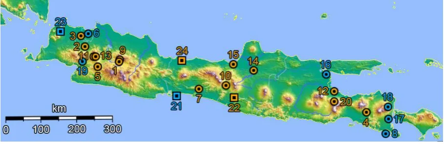
The study area of this research is the island Java, which is part of Indonesia. Java has a tropical climate. It basically has only two seasons; wet and dry. The wet season is from November until April and the dry season is from May until October. A map of the study area is shown in figure 3.1. In this map the locations of the 24 different measurement stations are shown (so these are not the locations of the cities, but the locations of the measurement stations at those cities). The locations shown in blue are boundary locations of the interpolation surface, meaning that they cannot be used as control data, for extrapolation would be needed then. Control data is data that is excluded when creating the interpolation surface, because it is used for validation of the model. This means that, when one of the boundary locations is taken away, the area over which can be interpolated becomes smaller, so the boundary locations determine the shape of the surface. The remaining locations are shown in orange. The locations marked with a square are locations with data supplied by BMKG and the locations marked with a circle are locations with data supplied by FAO.

= Data from FAO and a boundary location = Data from FAO and not a boundary location = Data from FAO and a boundary location = Data from FAO and not a boundary location

Measurement locations:

1. Bandung

2. Bogor

3. Curug-Budiarto 4. Djember 5. Gunung Rosa 6. Jakarta

7. Karang Anjar 8. Kawah-Idjen

9. Lembang

10. Magelang 11. Pangerango 12. Pasuruan

13. Rarahan 14. Sawahan 15. Semarang 16. Surabaya 17. Rogodjampi 18. Tamansari

19. Tjipetir 20. Tosari 21. Cilacap 22. Yogyakarta 23. Serang 24. Tegal

Figure 3.1: Map of Java with locations of the measurement stations

As can be seen in figure 3.1, the locations of the measurement stations are not very well distributed over the area. This means that in some areas because of this the interpolation will be better and in some areas it will be very bad. The biggest amount of measurement stations is located in the western part of Java. Two other ‘groups’ of measurement stations can be seen respectively in the middle and in the eastern part of Java. For making better interpolation possible between these ‘groups’ of measurement stations, data from more measurement stations will be needed.

3.2.

Meteorological data

14 supplied by the Indonesian National Agency for Meteorology, Climatology and Geophysics (BMKG). The data contains values for all variables listed in section 2.3.2. The following table shows the source of the data for all 24 measurement locations.

Number Location Source

1 Bandung FAO

2 Bogor FAO

3 Curug Budiarto FAO

4 Djember FAO

5 Gunung Rosa FAO

6 Jakarta FAO

7 Karang Anjar FAO

8 Kawah-Idjen FAO

9 Lembang FAO

10 Magelang FAO

11 Pengerango FAO

12 Pasuruan FAO

Number Location Source

13 Rarahan FAO

14 Sawahan FAO

15 Semarang FAO

16 Surabaya FAO

17 Rogodjampi FAO

18 Tamansari FAO

19 Tjipetir FAO

20 Tosari FAO

21 Cilacap BMKG

22 Yogyakarta BMKG

23 Serang BMKG

24 Tegal BMKG

Table 3.1: Locations of the used measurement stations and the source of their climate data

FAO data

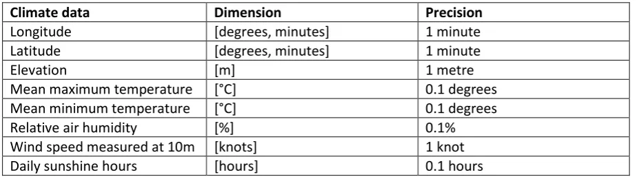
The data from FAO comes from a climatic database called “CLIMWAT” (FAO, 1994). This database was published in 1994, so the climate data in it is quite old. The database contains monthly values for the variables used as model input. These monthly values are averaged over years of climatic data. The individual values for these years however are not given in the database. Table 3.2 below shows in which dimensions and with which precisions this data is given.

Climate data Dimension Precision

Longitude [degrees, minutes] 1 minute

Latitude [degrees, minutes] 1 minute

Elevation [m] 1 metre

Mean maximum temperature [°C] 0.1 degrees

Mean minimum temperature [°C] 0.1 degrees

Relative air humidity [%] 1%

Wind speed measured at 2m [km day-1] 1 km/day

Daily sunshine hours [hours] 0.1 hours

Table 3.2: Dimensions and precision of the FAO climate data

BMKG data

The data from BMKG was given in an Excel sheet. In this sheet, data was given for the years 2000 to 2006 for every month. In the model the average from the years 2000 until 2006 is used as input. Table 3.3 below shows in which dimensions and with which precisions this data is given.

Climate data Dimension Precision

Longitude [degrees, minutes] 1 minute

Latitude [degrees, minutes] 1 minute

Elevation [m] 1 metre

Mean maximum temperature [°C] 0.1 degrees

Mean minimum temperature [°C] 0.1 degrees

Relative air humidity [%] 0.1%

Wind speed measured at 10m [knots] 1 knot

Daily sunshine hours [hours] 0.1 hours

15

Longitude and latitude data

The precision of the longitudes and latitudes given are 1 minute. This is equal to about 1.85 kilo-meters. On a national scale this is not a big deal, but on a local scale it matters quite much. The model is supposed to be used by farmers on a local scale, so the coordinates should be given with a higher precision in the future.

Wind speed data

The wind speed data supplied by FAO does not seem to be correct for all the measurement stations. The wind speeds are very low compared to the wind speeds in the BMKG data. Sometimes the measured wind speed does not even vary during the year. This means that the dependence between the wind speed and the variations of the reference crop evapotranspiration does not apply at those locations. This probably did not make the result of the model better, but no better wind data was available during the course of this study. The wind speed in knots measured at 10 meters height was converted to the wind speed in [m s-1] measured at 2 meters height. Probably the differences are due to different ways of measuring.

The conversion from knots at 10 meters height ( ) to meters per second at 2 meters height ( ) was done in the following way. One knot is equal to exactly 1.852 km/h and one m/s is equal to exactly 3.6 km/h, so equation 3.1 below is used to get from the wind speed in knots to the wind speed in m/s at 10 meters height ( ):

(eq. 3.1)

Then the wind speed in m/s at 10 meters height needs to be converted into the wind speed in m/s at 2 meters height. This is done by using a conversion factor from Annex 2 in Allen et. al. (1998). This conversion factor is calculated as shown in equation 3.2. In this equation is the original height of the measurement, so in this case 10. The calculated conversion factor is then multiplied with the wind speed in m/s at 10 meters height to come to the wind speed in m/s at 2 meters height, as shown in equation 3.3.

(eq. 3.2)

(eq. 3.3)

3.3.

Elevation data

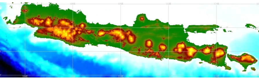
In this research altitude data of the research area was also used. This data has been provided through the GEBCO Grid Display software (GEBCO, 2009). GEBCO’s main goal is providing bathymetric charts of the oceans, but they also have data of the altitudes over land. The land data is largely derived from the Shuttle Radar Topography Mission (SRTM30) data set. The data has 30 arc-seconds spacing, which is about 0.92 kilometers. Considering that the longitudes and latitudes provided by the measurement stations are provided with an accuracy of 60 arc-seconds, the spacing of this altitude data should be accurate enough.

16

Figure 3.2: Altitude data of Java with 30 arc-seconds spacing.

17

4.

Modeling and interpolation methods

In this research various methods have been used to interpolate the . In total 5 methods have been used. The first method is just plainly interpolating the . In the second method the was split up into three components; , and . Here and were interpolated and the measured wind speed was used after the interpolation. In the third method the was split up into five components; , , , and . Here , , and were interpolated and the measured wind speed was used after the interpolation. In the third method, none of the interpolated components contain anywhere, while and still contained in the second method. The fourth method is the same as the third method, except for that the is not interpolated, but calculated using the GEBCO elevation data. The fifth method is also the same as the third method, except for that the is not interpolated, but calculated using the altitude given in the data from the measurement locations. For each of these methods the results were obtained in the following way. For every station not on the boundary the model was run thirteen times, once for each month and once for the average over the year. When the model is run for a certain station, this means that this certain station is left out in the interpolation process and the data of that station is thus used as control data (used for validation). It has been chosen to only take one station as a control point at a time, because of the small amount of measurement locations with available data. However, with the model it is possible to take multiple stations as control points in the same run.

Now the different methods will be explained in more detail.

4.1.

Interpolation methods in MatLab

The interpolation is done using the griddata function in MatLab, this function can use 4 different interpolation methods. These four methods are:

triangle-based linear interpolation triangle-based cubic interpolation nearest neighbor interpolation the MATLAB v4 griddata method

18

4.2.

Modeling methods

In the sub-paragraphs of this paragraph (4.2.1 to 4.2.5) the details of the 5 different methods are given. For each method is first explained in which components the is divided in these sub-paragraphs.

In Method 1, first the is calculated for each point that is not a control point. In Methods 2 to 5, first the values of the components are calculated for each point that is not a control point. Then there are a certain amount of points that have coordinates (longitude and latitude) and a value for the components (and in Method 1 for the ). These points are then used to make interpolation surfaces, one for each of the components (and in Method 1 for the ). The interpolation surfaces are actually a gridded matrices with values of the different components or the in them. The interpolations are done separately for each month and also for the averaged values over the year.

The values for the components and the are also calculated for the control points, but these were not used to generate the interpolation surfaces. Then the coordinates of the control points are used to find the predicted value of the components (and in Method 1 of the ) for the control points in the gridded matrices. In Methods 2 to 5 the value for is taken from the measurement data at the control point. This is because when the model is ready, the predicted wind speed can be entered in the model here.

When there is a control point , which has location ( , ), where and are the longitude and latitude in decimal degrees respectively. Then the predicted at control point in a specific month can approximately be determined. Approximately, because the exact values of and are not always on the axes of the interpolation surface, but the nearest points on the axes are taken. The equation for calculating the predicted for each method is given in the sub-paragraph of that method. The values of the predicted and the as calculated using all the measurement data at the control point can then be compared.

4.2.1. Method 1: Interpolating the ETo

In this model the FAO-56 Penman-Monteith equation (equation 2.8) is used to calculate the . In this method the as calculated by this equation is interpolated directly.

In this method, the predicted at control point in a specific month is approximately given by:

(eq. 4.1)

4.2.2. Method 2: The α and β method

The FAO-56 Penman-Monteith equation (equation 2.8) can be written in the following form:

(eq. 4.2)

Where:

(eq. 4.3)

(eq. 4.4)

: measured wind speed at 2 m height [m s-1]

19 In this method we assume that we have a prediction of the wind speed in month at point in noted as . Then the predicted at control point in month is approximately given by:

(eq. 4.5)

4.2.3. Method 3: The abcd method

The FAO-56 Penman-Monteith equation (equation 2.8) can be written in the following form:

(eq. 4.6)

Where:

(eq. 4.7)

(eq. 4.8)

: psychrometric constant [kPa °C-1]

: slope of the relationship between the saturation vapor pressure and temperature [kPa °C-1] : measured wind speed at 2 m height [m s-1]

In this method , , and are the components which are interpolated separately. This method is called “The abcd method” because the first four letters in the Greek alphabet are interpolated. The main goal of this method was to exclude entirely from the interpolation, because and did still contain in their equations (equations 4.3 and 4.4).

In this method we assume that we have a prediction of the wind speed in month at point in noted as . Then the predicted at control point in month is approximately given by:

(eq. 4.9)

Where:

(eq. 4.10)

(eq. 4.11)

(eq. 4.12)

(eq. 4.13)

Note that the predicted does not depend on the month, this is because only depends on the altitude, which doesn’t change during the year.

4.2.4. Method 4: The abcd method, but using altitude data for determining γ

This method is the same as Method 3, except for the fact that the is determined in another way. The elevation data from GEBCO (see section 3.3) is used to calculate the values for . In figure 2.1 can be seen that only depends on the altitude. This can also be seen in equations 2.22 and 2.23.

20 (eq. 4.14)

As described in paragraph 3.3, altitude data of Java was available for this research. This altitude data can be put into a matrix. Assume this matrix contains rows and columns, then every cell of the matrix contains an altitude . Now equation 4.14 can be used to make a in the following way:

(eq. 4.15)

If this is done for from 1 to the amount of rows in the altitude matrix and for from 1 to the amount of columns in the altitude matrix, is obtained. With this new equation 4.9 and the underlying equations (4.10 until 4.13) can be applied to obtain the new predicted values for

at the control points.

4.2.5. Method 5: The abcd method, but using the given height to determine γ

This method is the same as Method 3, except for the fact that the is not predicted. In this method the assumption is made that the altitude belongs to the input of the model. When the longitude and latitude can be given, then it might be a small step to also add the altitude to that. This means there will be no error due to in the predicted .

In this method the predicted at control point in month is approximately given by:

(eq. 4.16)

Where:

(eq. 4.10)

(eq. 4.11)

(eq. 4.17)

21

5.

Results and discussion

In this chapter the results of the research are shown. The results will be discussed for every method. The results will be looked at from a per month view and a per station view. After the results are shown, the results will be discussed in more detail.

5.1.

Results

In the results mostly errors are shown. Errors are interesting, because they show how good the interpolation is in comparison to the calculation from measurements. The error is defined as the relative difference between the predicted values and the values as calculated from measurements (CfM). The errors are calculated in the following way:

(eq. 5.1)

This means that when the error is positive, the predicted value is higher than the value as calculated from measurements. When the error is negative, the predicted value is lower than the value as calculated from measurements.

All errors as shown here are errors in the . For example, when an error is called “Error due to error in alpha”, this means that the is calculated in two ways. In the case of the error due to alpha in Method 2 (the and method), the “predicted value” and “value as calculated from measurements” in equation 5.1 are calculated in the following way:

(eq. 5.2)

(eq. 5.3)

5.1.1. Monthly errors

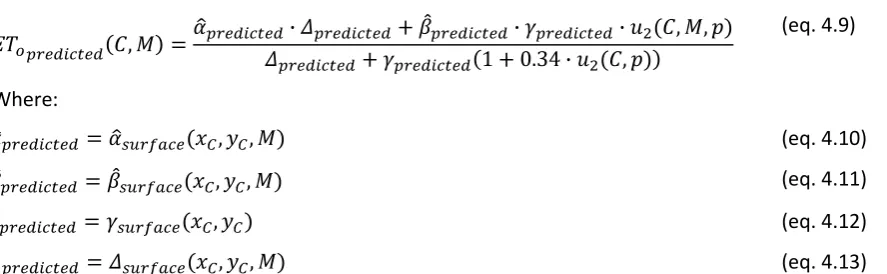
First the errors will be shown per month for every method. The errors shown in this paragraph (5.1.1) are all averaged over all the stations used as control points. The monthly errors for Method 1 with both linear and cubic triangle-based interpolation are shown in figure 5.1 below.

Figure 5.1: Method 1 - monthly errors for linear and cubic interpolation

The errors shown in figure 5.1 are absolute errors, this means that only the size of the error is displayed and not if the error is positive or negative. This is done because the errors become very small when averaging positive and negative errors, so then they don’t give a good representation of the results. As can be seen, the error with cubic interpolation is bigger than the error with linear interpolation for each month. The errors are the biggest in October and November with 21,4% and 21,0% respectively for cubic and 19,6% and 19,5% respectively for linear.

0% 5% 10% 15% 20% 25%

1 2 3 4 5 6 7 8 9 10 11 12

ab

solut

e

e

rr

o

r

in

E

To

(%

)

Month

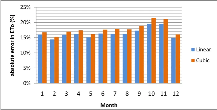
22 For Method 2, the alpha and beta method, the distribution of monthly errors looks different. The monthly errors for Method 2 with both linear and cubic triangle-based interpolation are shown in figure 5.2 below.

Figure 5.2: Method 2 - monthly errors for linear and cubic interpolation

The errors shown in figure 5.2 are also absolute errors. As can be seen, again the error with cubic interpolation is bigger than the error with linear interpolation for each month. Because cubic triangle-based interpolation was worse for every month and over 70% of the measurement stations used as control points in both Method 1 and 2, this method is not used in Methods 3, 4 and 5. On average, the errors of Method 2 are bigger than the errors of Method 1. The average errors of each method are presented in the paragraph named “Average errors per method”. The errors are the biggest in January, February and November with 20.9%, 22.1% and 21.4% respectively for cubic and 20.5%, 21.1% and 20.3% respectively for linear.

The influence of alpha and beta to the error in is also an interesting thing to look at in this method. The error due to alpha is the error in that occurs when the error in beta is set to zero and the error due to beta is the error in that occurs when the error in alpha is set to zero. Figure 5.3 shows the absolute errors due to alpha and beta with linear interpolation.

Figure 5.3: Method 2 - monthly errors due to alpha and beta for linear interpolation 0%

5% 10% 15% 20% 25%

1 2 3 4 5 6 7 8 9 10 11 12

ab

solut

e

e

rr

o

r

in

E

To

(%

)

Month

23 The errors shown here are absolute errors, this means only the size of the error is shown and not if the errors are negative or positive. As can be seen, the biggest part of the error in the is caused by errors in alpha. Also, the error due to alpha varies more during the year than the error due to beta. The error in the in November is mainly caused by the error in alpha, because the error in beta is actually very low here, while this month has one of the highest errors in the .

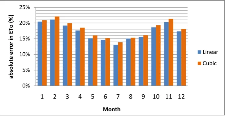
For methods 3, 4 and 5, the distribution of monthly errors looks a lot like the distribution of errors in Method 1. The monthly errors in the for Methods 3, 4 and 5 with only linear triangle-based interpolation are shown in figure 5.4 below.

Figure 5.4: Methods 3, 4 and 5 - monthly errors for linear interpolation

The errors shown in figure 5.4 are also absolute errors. As can be seen, the errors of Method 4 are larger than the errors of Method 3 and the errors of Method 5 are even bigger. On average, the errors of Methods 3, 4 and 5 are smaller than the errors of Method 1. This means that of all the methods, Method 3 has the smallest errors in the . The errors are the biggest in October and November (like in Method 1), with 17.8% and 17.3% respectively for Method 3, 19.2% and 19.0% respectively for Method 4 and 19.3% and 19.1% respectively for Method 5.

The influence of , , and to the error in is also an interesting thing to look at in these three methods. Figures 5.5, 5.6 and 5.7 show the absolute errors due to , , and respectively. The error due to the error in a certain component is the error in that occurs when the errors in all other components are set to zero.

Figure 5.5: Method 3 (linear) - monthly errors due to alpha, beta, gamma and delta

0% 2% 4% 6% 8% 10% 12% 14% 16% 18% 20%

1 2 3 4 5 6 7 8 9 10 11 12

ab so lu te er ro r in ET o ( %) Month Method 3 Method 4 Method 5 0% 2% 4% 6% 8% 10% 12% 14% 16% 18% 20%

1 2 3 4 5 6 7 8 9 10 11 12

ab solut e e rr o r in E To (% ) Month

Error in ETo

24

Figure 5.6: Method 4 (linear) - monthly errors due to alpha, beta, gamma and delta

Figure 5.7: Method 5 (linear) - monthly errors due to alpha, beta and delta

As can be seen, the biggest part of the error in the is caused by errors in . Also, only the errors due to and seem to change significantly during the year. The error in gamma does not change during the year at all, because it only depends on the altitude in this model. The error in delta does not change much, because it depends on the temperature, which does not vary much during the year in Java. The error due to the error in gamma decreases from Method 3 to Method 4, but this makes the total error in the increase. This is because effect of the error in gamma to the value of the is positive when the effect of the errors in the other components to the value of the are negative and vice versa. When the error in gamma is taken away partially (in Method 4), the absolute error in increases. When the error in gamma is taken away entirely (in Method 5), the absolute error in increases even further. In Methods 4 and 5 however, the sum of absolute errors in the components is smaller.

5.1.2. Errors per station

Here the errors will be shown for every station not on the boundary (the stations marked with an orange circle or square in figure 3.1). The errors shown in this paragraph (5.1.2) are all averaged over the year. The errors per station for Method 1 with both linear triangle-based interpolation are shown in figure 5.8 below.

0% 2% 4% 6% 8% 10% 12% 14% 16% 18% 20%

1 2 3 4 5 6 7 8 9 10 11 12

ab solut e e rr o r in E To (% ) Month

Error in ETo

Absolute error due to error in alpha Absolute error due to error in beta

0% 2% 4% 6% 8% 10% 12% 14% 16% 18% 20%

1 2 3 4 5 6 7 8 9 10 11 12

ab solut e e rr o r in E To (% ) Month

Error in ETo

25

Figure 5.8: Method 1 - errors for each station averaged over the year for linear interpolation

As can be seen, station 20 (Tosari) has a very large error of 61.5%. Why this is will be discussed in section 5.2. Stations 14 (Sawahan) and 15 (Semarang) however show very small errors, 2.7% and -1.3% respectively.

The distribution of errors over the stations looks very different in Method 2. The errors per station for Method 2 with linear triangle-based interpolation are shown in figure 5.9 below.

Figure 5.9: Method 2 - errors per station for linear interpolation

It can be seen that, like in Method 1, stations 14 (Sawahan) and 15 (Semarang) show very small errors and station 20 (Tosari) shows very high errors. In comparison with Method 1, stations 7, 10, 11, 14, 22 and 24 show a sign change. In this method, the error at station 11 (Pangerango) is also very high, why this is will also be discussed in section 5.2. The errors at stations 11 and 20 are 47.0% and 48.4% respectively. In the graphs the errors due to the errors in alpha and beta are also shown. For every station, except for station 15 where the total error is very small, the error due to alpha is much bigger than the error due to beta. The errors in alpha generate about 81% of the error in the

. -30% -20% -10% 0% 10% 20% 30% 40% 50% 60%

1 2 3 4 5 7 9 10 11 12 13 14 15 20 22 24

Er

ro

r

in

E

To

(

%)

Stations

26 The distribution of errors over the stations looks a bit different in Methods 3, 4 and 5. The errors per station for Methods 3, 4 and 5 are respectively shown in figures 5.10, 5.11 and 5.12 below.

Figure 5.10: Method 3 - errors per station for linear interpolation

Figure 5.11: Method 4 - errors per station for linear interpolation

-30% -20% -10% 0% 10% 20% 30% 40% 50% 60%

1 2 3 4 5 7 9 10 11 12 13 14 15 20 22 24

Er

ro

r

in E

T

o

(

%)

Stations

Error due to error in gamma Error due to error in delta Error due to error in beta Error due to error in alpha Total error

-30% -20% -10% 0% 10% 20% 30% 40% 50% 60%

1 2 3 4 5 7 9 10 11 12 13 14 15 20 22 24

Er

ro

r

in

E

To

(

%)

Stations

27

Figure 5.12: Method 5 - errors per station for linear interpolation

Again, stations 11 and 20 show very high errors. But most of the other stations show lower errors in these methods. ”. The errors at stations 11 and 20 are 34.4% and 53.2% respectively for Method 3, 39.7% and 58.8% respectively for Method 4 and 41.4% and 58.6% respectively for Method 5. In figure 5.10 can be seen that in Method 3, the error due to the error in gamma is often negative when all the other errors are positive and vice versa. This means that when the error due to gamma is reduced, as in Methods 4 and 5, the absolute error in the becomes higher. Table 5.1 below shows the share of alpha, beta, gamma and delta in the error of the in Methods 3, 4 and 5.

error due to error in

error due to error in

error due to error in

error due to error in Method 3 36.8% 33.5% 9.2% 20.5%

Method 4 39.4% 35.4% 1.8% 23.4%

Method 5 39.9% 36.0% 0.0% 24.1%

Table 5.1: The share of alpha, beta, gamma and delta in the error of the in Methods 3, 4 and 5

In all methods, the errors in cause the biggest part of the error in the . The errors in also cause a big part of the error in the .

5.1.3. Average errors per method

In this paragraph will be looked at the average errors the different methods produce. The average errors of the different methods are shown in table 5.2 below.

Method 1 Method 2 Method 3 Method 4 Method 5

Linear Cubic Linear Cubic Linear Linear Linear

16.5% 17.8% 17.3% 18.1% 14.8% 16.3% 16.4%

Table 5.2: The average errors of the different modeling methods with the different interpolation methods

As can be seen, Method 3 is showing the best results. Method 2 actually has bigger average errors than Method 1, so the alpha and beta method is not better than just plain interpolation with the data used in this research. Methods 3, 4 and 5 are all better than Method 1.

In figures 5.8, 5.9, 5.10, 5.11 and 5.12 can be seen that the error in stations 11 and 20 is often much higher than the average error. This may mean the interpolation in these points makes not much

-30% -20% -10% 0% 10% 20% 30% 40% 50% 60%

1 2 3 4 5 7 9 10 11 12 13 14 15 20 22 24

Er

ro

r

in

E

To

(

%)

Stations

28 sense with the used methods. A method can have a very low average error just because it makes the error in these bad points better, while it could at the same time create a worse result in the remaining points. Also, a method can have a very high average error just because it makes the error in the bad points worse, while it could at the same time create a better result in the remaining points. This means it makes sense to look at the average error of all stations except for 11 and 20. The average errors of the different method with exclusion of the errors in stations 11 and 20 are shown in table 5.3 below.

Method 1 Method 2 Method 3 Method 4 Method 5

Linear Cubic Linear Cubic Linear Linear Linear

12.3% 13.6% 13.0% 13.9% 10.5% 11.4% 11.5%

Table 5.3: The average errors of the different modeling methods with the different interpolation methods

As can be seen, the order in Methods, from good to bad, remains the same. It looks like it is just coincidence that Method 3 is better than Methods 4 and 5, which means it might be that Methods 4 and 5 are better when using other data sets, for instance with climatic data from different measurement stations or in a different research area.

5.1.4. Monthly variations

Here the monthly variations of alpha and beta for Method 2 and the monthly variations of , , and for Methods 3, 4 and 5 will be shown. This is interesting, because if the monthly variation is very low, an average interpolation over the year could be sufficient. When this is the case, the model can be made more simple. The values given in this paragraph are all calculated from only measurements, so no interpolation methods apply here.

In figure 5.13 below the monthly values of alpha are given for Method 2 for each station.

Figure 5.13: Method 2 - values of alpha for each station at each month

In figure 5.13 can be seen that the alpha fluctuates quite much during the year. On average (averaged per station), the maximum values are 15.8% bigger than the average values (averaged over the year). The minimum values are on average 14.4% smaller than the average values. This means the average difference between the minimum and the maximum value lies about 30.2% around the average, which is quite high. This is logical, because as can be seen in equation 4.3, alpha depends on , which does not only depends on the temperature, but also on the daily sunshine hours and the number of the day in the year. The sunshine hours have a higher variation than the temperature.

0 0,5 1 1,5 2 2,5 3 3,5 4 4,5 5

1 2 3 4 5 6 7 8 9 10 11 12

α

Month

29 In figure 5.14 below the monthly values of beta are given for Method 2 for each station.

Figure 5.14: Method 2 - values of beta for each station at each month

In figure 5.14 can be seen that beta fluctuates even more than alpha during the year. On average, the maximum values are 29.1% bigger than the average values. The minimum values are on average 24.0% smaller than the average values. This means the average difference between the minimum and the maximum value lies about 53.1% around the average, which is very high. The relative differences are big, but the absolute differences are not very big, because beta has a very low value. The monthly variations are quite big because beta does not only depend on the temperature, but also on the relative humidity.

In figure 5.15 below the monthly values of are given for Methods 3, 4 and 5 for each station.

Figure 5.15: Methods 3, 4 and 5 - values of for each station at each month -0,1

6E-16 0,1 0,2 0,3 0,4 0,5 0,6 0,7

1 2 3 4 5 6 7 8 9 10 11 12

β

Month

Station 1 Station 2 Station 3 Station 4 Station 5 Station 7 Station 9 Station 10 Station 11 Station 12 Station 13 Station 14 Station 15 Station 20 Station 22 Station 24

0 1 2 3 4 5 6 7

1 2 3 4 5 6 7 8 9 10 11 12

α

ˆ

Month

30 As can be seen, fluctuates about as much as alpha did. On average, the maximum values are 15.1% bigger than the average values. The minimum values are on average 13.5% smaller than the average values. This means the average difference between the minimum and the maximum value lies about 28.6% around the average, which is again quite high. The monthly variations are a bit smaller, because does not at all depend on the wind speed (equation 4.7).

In figure 5.16 below the monthly values of are given for Methods 3, 4 and 5 for each station.

Figure 5.16: Methods 3, 4 and 5 - values of for each station at each month

As can be seen, also fluctuates about as much as beta did. On average, the maximum values are 31.3% bigger than the average values. The minimum values are on average 25.2% smaller than the average values. This means the average difference between the minimum and the maximum value lies about 56.5% around the average, which is again very high. The monthly variations are a bit larger, probably because the variations in the relative humidity and the temperature contributed more to the variation in beta than the variations in delta and the wind speed.

In figure 5.17 below the monthly values of are given for Methods 3, 4 and 5 for each station.

Figure 5.17: Methods 3, 4 and 5 - values of Δ for each station at each month 0

0,5 1 1,5 2 2,5 3 3,5 4

1 2 3 4 5 6 7 8 9 10 11 12

β

ˆ

Month

Station 1 Station 2 Station 3 Station 4 Station 5 Station 7 Station 9 Station 10 Station 11 Station 12 Station 13 Station 14 Station 15 Station 20 Station 22 Station 24

0 0,05 0,1 0,15 0,2 0,25

1 2 3 4 5 6 7 8 9 10 11 12

Δ

[kPa/

C]

Month

31 As can be seen, does not fluctuate very much over the year. On average, the maximum values are only 4.5% bigger than the average values. The minimum values are on average only 5.9% smaller than the average values. This means the average difference between the minimum and the maximum value lies about 10.4% around the average, which is not very high. This means using only one surface where the average values over the year are used may be sufficient for , as it will only create an error of about 5.2% in on average. It is quite logical that the variation in is very low, because (as can be seen in equation 2.9) it only depends on the temperature, which doesn’t vary very much in Indonesia.

5.2.

Discussion

In this section the phenomena seen in the results and the limitations of this study will be discussed. Based on this discussion, in the next chapter recommendations for improving the model and for further research will be given. The recommendations can be found in section 6.2.

The results showed that the error in the in Method 1 was smaller than in Method 2. This is most probably due to the fact that the error that is created by not (partially) excluding the wind speed from the interpolation in Method 1 actually makes the error in the predicted smaller. It could be that with a different research area or with data from different measurement stations the results of Method 2 are better than those of Method 1.

As can be seen in section 3.1, data was available for only 24 measurement stations and it looked like the wind data from the two different data suppliers was measured in a different way. Also, for some stations the measured wind speed was the same for the whole year, which may mean that only a rough estimate is given. The concept of the model relies on the dependency of the to the wind speed, so this probably did not influence the results in a good way. The amount of available measurement locations with the needed data was actually too little for a study area as big as whole Java. Retrieving more measurement data was too costly and took too much time for this research, but maybe this can be done in a following research.

In the previous section the results were discussed. It could be seen that the errors of the stations Pangerango and Tosari were very high. When looking at why this may be, we saw that these stations are both quite high up in the mountains, the station at Pangerango has an altitude of 3023m and the station at Tosari has an altitude of 1735m. In figures 5.10, 5.11 and 5.12 can be seen that the stations at Pangerango and Tosari both have a rather high error in the due to the error in delta. The equation used for calculating delta (equation 2.9) shows that delta only depends on one variable, the mean temperature. Of course high up in the mountains it is much colder than at sea level. Also, the stations at Pangerango and Tosari are very close to other stations with lower altitudes; Pangerango is very close to Rarahan which has an altitude of 1400 m and Tosari is very close to Pasuruan which has an altitude of only 5 m. This is most probably the origin of the big errors at stations 11 and 20, because the predicted values will be very close to the value at the closest station when stations 11 and 20 are used as control points. Also, around stations 11 and 20 there are multiple stations with a lower altitude compared to them, which also explains why the stations around 11 and 20 don’t have such big errors.

32 gamma (up to a certain level) actually creates a model with a better validation result. In section 7.2 will be explained why Method 3 is not really the best method to build up on, when an improvement is to be made to the model.

33

6.

Conclusions and recommendations

6.1.

Conclusions

The main goal of this research was to develop and apply a model for determining the reference crop evapotranspiration ( ) for Java spatially and temporally distributed. This had to be done by using different interpolation methods where the predicted wind speed is used as input. It can be said that this goal is achieved, because the model can determine the spatially distributed over Java and for each month. The last methods (Method 4 and 5), which entirely exclude the wind speed from the interpolation showed the best result, which shows that it makes sense to use the predicted wind speed as input for the model.

The results of this research showed that for the interpolation used in this model, linear triangle-based interpolation gives better results than cubic triangle-triangle-based interpolation. Cubic interpolation may look better, but it does not give more reliable results, because the smoothness is not based on anything physical.

The research also showed that plain interpolation is still better than the alpha and beta method. This is probably because errors cancel each other out in Method 1. This could be just coincidence, meaning that Method 2 could actually be better when using different data sets. However, Methods 3, 4 and 5 are better than plain interpolation. In Methods 3, 4 and 5, the wind speed is entirely excluded from the interpolation process. Of these three methods, Method 3 shows the best results, but this is due to the fact that errors cancel each other out here.

The research also showed that it is very hard to get enough and reliable data in Indonesia. This limited this research quite a bit, because with data from more stations the interpolation could have been carried out in more detail, which probably would have revealed more flaws and options of the model. As can be seen in figure 3.1, the locations of the measurement stations used in this research were quite clustered, so the model does not really give a good estimation of the over whole Java island. Retrieving more data has been tried during the course of this research, but with no success. Retrieving the data takes long, because the data is not stored digitally, so it needs to be prepared. Also, it is hard to find the people who actually have access to the data.

The model currently does not take into account the temperature decrease at high altitudes. This resulted in high errors at locations with low distance to neighboring stations as the crow flies, but with high altitude differences.

34

6.2.

Recommendations

In this section recommendations will be given for a possible following research.

The method with the best results was Method 3 in this research, but this does not mean this is the model that should be improved. The errors in the were only lower due to the fact that errors cancel each other out in this method (see the description below figures 5.10, 5.11 and 5.12). When improving the model, either the errors in Method 4 or Method 5 should be reduced, to be able to obtain the best results, because the sum of absolute errors in the components is lower in these methods. If it is realistic to include the altitude of the location in the input for the model for points not used in the interpolation, Method 5 should be used, otherwise Method 4 is better. This is realistic if it is easy and accurate to measure the altitude with a GPS device, for instance.

As said in section 6.1., the model currently does not take into account the temperature decrease when the altitude increases. The variables still creating much of the errors in the in Methods 4 and 5 are , and . In equation 4.7 can be seen that depends on and . In equation 4.8 can be seen that depends on , and . In equation 2.9 can be seen that depends on . Figure 2.1 shows that , , and all depend on the temperature. This means that when the temperature is interpolated in a better way, the errors in , and could all decrease. However, it is not an easy job to interpolate the temperature in such a way that it takes into account the altitude, because all known temperatures are all already measured at a certain altitude, so the difference between the altitude at the measurement locations and the altitude at the interpolation points should be taken into account. This means can use the temperatures of some kind of temperature surface, because it is only directly related to the temperature. For , and need to be substituted by their equations to make directly related to the temperature. Also, for , and need to be substituted by their equations to make directly related to the temperature.

For a following research it is also recommended that first more data is obtained. Data of much more stations is needed to make the interpolation over whole Java island better. In figure 3.1 can be seen that the current measurement stations with available data do not cover whole Java island. Especially near the south coast more data from measurement stations is needed. What also can be done, is checking out if a standardization of the Penman-Monteith formula can be made for locations near the shoreline. Maybe certain conditions are always the same near the shoreline, which may mean that it is possible to make an equation for calculating the near the shoreline that only depends on the location of the point on the shoreline and not on any local meteorological measurements. If this is possible, then the shoreline can be used as a boundary and over whole Java the values for the

35

References

Allen, R., Pereira, L., Raes, D., & Smith, M. (1998). Crop evapotranspiration - Guidelines for computing crop water requirements - FAO Irrigation and drainage paper 56. Rome: FAO - Food and Agriculture Organization of the United Nations.

Bulsink, F. (2008). The Water Footprint of Indonesian Provinces - The relation between water use and consumption in Indonesian provinces. Enschede: University of Twente.

Case, M., Ardiansyah, F., & Spector, E. (2007). Climate Change in Indonesia - Implications for humans and nature. WWF.

FAO. (1994). FAO - Water Development and Management Unit - Information Resources - Databases. Retrieved July 25, 2009, from Website of FAO:

http://www.fao.org/nr/water/infores_databases_climwat.html

FAO. (2009). FAO - Water Development and Management Unit - Information Resources - Software. Retrieved September 3, 2009, from Website of FAO:

http://www.fao.org/nr/water/infores_databases_cropwat.html

GEBCO. (2009, May 21). Release of the GEBCO_08 Grid. Retrieved June 30, 2009, from GEBCO website: http://www.gebco.net/about_us/news_and_events/gebco_08_release.html

IPCC. (2007, november). Climate Change 2007: Synthesis Report - Summary for Policymakers. Valencia, Spain.

Olchev, A., Ibrom, A., Priess, J., Erasmi, S., Leemhuis, C., Twele, A., et al. (2008). Effects of land‐use changes on evapotranspiration of tropical rain forest margin area in Central Sulawesi (Indonesia): Modelling study with a regional SVAT model. Ecological Modeling 212 , 131-137.

Safrina, M. (2009, June 25). The tale of the `Emerald of the Equ