Optimal Reciprocal Reinsurance under GlueVaR Distortion Risk Measures

(1)

ISSN Online: 2162-2442 ISSN Print: 2162-2434

DOI: 10.4236/jmf.2019.91002 Jan. 17, 2019 11 Journal of Mathematical Finance

Optimal Reciprocal Reinsurance under

GlueVaR Distortion Risk Measures

Yuxia Huang, Chuancun Yin

School of Statistics, Qufu Normal University, Qufu, China

Abstract

This article investigates the optimal reciprocal reinsurance strategies when the risk is measured by a general risk measure, namely the GlueVaR distor-tion risk measures, which can be expressed as a linear combinadistor-tion of two tail value at risk (TVaR) and one value at risk (VaR) risk measures. When we consider the reciprocal reinsurance, the linear combination of three risk measures can be difficult to deal with. In order to overcome difficulties, we give a new form of the GlueVaR distortion risk measures. This paper not only derives the necessary and sufficient condition that guarantees the optimality of marginal indemnification functions (MIF), but also obtains explicit solu-tions of the optimal reinsurance design. This method is easy to understand and can be simplified calculation. To further illustrate the applicability of our results, we give a numerical example.

Keywords

Distortion Risk Measure, VaR, TVaR, GlueVaR, Marginal Indemnification Function (MIF), Optimal Reciprocal Reinsurance

1. Introduction

Reinsurance is an effective risk management tool for the insurer to transfer part of its risk to the reinsurer. Let X be the original loss, if the insurer cedes a part of loss f X

( )

(f is called the ceded loss function, or indemnification function) to the reinsurer and pays reinsurance premium

δ

f

( )

X , then the insurer’s total

liability TI_f

( )

X contains two parts: one is the retained loss risk

( )

f

I X = −X f X and the other is the reinsurance premium

δ

f

( )

X , that is

( )

.

f

I f

T X = X f X− +δ X (1.1)

The reinsurer’s total liability TR_f

( )

X also contains two parts: one is the

How to cite this paper: Huang, Y.X. and Yin, C.C. (2019) Optimal Reciprocal Rein-surance under GlueVaR Distortion Risk Measures. Journal of Mathematical Finance, 9, 11-24.

https://doi.org/10.4236/jmf.2019.91002

Received: December 16, 2018 Accepted: January 14, 2019 Published: January 17, 2019

(2)

DOI: 10.4236/jmf.2019.91002 12 Journal of Mathematical Finance

ceded loss risk

R X

f

( )

=

f X

( )

and the other is the received reinsurance

pre-mium

δ

f

( )

X , that is

( )

.

f

R f

T X = f X −δ X (1.2)

For any

λ

∈

[ ]

0,1 , we define total risks T Xf

( )

in the presence of an insurer

and a reinsurer as

( )

_f

( ) (

1

)

_f

( )

.

f I R

T X =λT X + −λ T X _(1.3)

Due to the development and application of risk measures in finance and in-surance, many workers formulate the optimal reinsurance problem with Value at Risk (VaR) and Tail Value at Risk (TVaR). [1] proposed two optimization criterion that minimize total loss of the insurer by the Value at Risk (VaR) and the Conditional Tail Expectation (CTE). [2] showed that quota-share and stop-loss reinsurance are optimal when they studied a class of increasing convex ceded loss functions by VaR and CTE under the expected value principle. Many works extended the fundamental results, for example, [3]-[15]. [16] extended the conclusion of [15] to the general convex risk measure that satisfied regular inva-riance. Recently, there has a surge of interest in more generally distortion risk measures. [17] discussed the general model of the distortion risk measure and assumed that the distortion function is piecewise convex or concave. [18] stu-died the general model with distortion risk measures under general reinsurance premium principles. [19] expended the model of [18] under the cost-benefit framework. [20] studied the optimal reinsurance model of [18] without the pre-mium constraint by a marginal indemnification function (MIF) formula. [21] studied the optimal reinsurance with premium constraint by combining the MIF formula and the Lagrangian dual method. [22] and [23] studied the optimal reinsurance with constraints under the distortion risk measure.

VaR has been adopted as the standard tool for assessing the risks and calcu-lating the capital requirements in finance and insurance, however, it has two drawbacks in financial industry. One is that the capital requirements can be un-derestimated and the unun-derestimated may be aggravated when heavy tail losses are incorrectly modeled by mild tail distribution. The second one is that the VaR may fail the subadditivity. Though TVaR has no these two disadvantages of VaR, it has not been widely accepted by practitioners in finance and insurance. In or-der to overcome this weakness, [24] proposed a new family of risk measures, namely GlueVaR distortion risk measures. We take different definitions of VaR from [24], therefore, a new definition of GlueVaR has been given in this paper.

(3)

rein-DOI: 10.4236/jmf.2019.91002 13 Journal of Mathematical Finance

surance strategy under GlueVaR distortion risk measures with MIF formula. The rest of this paper is organized as follows. In Section 2, we give some nota-tions and proposal a reciprocal reinsurance model. In Section 3, we derive the sufficient conditions that guarantee the existence of a reinsurance contract. In Section 4, we obtain the specific expression of optimal reinsurance. Section 5 concludes this paper.

2. The Model

2.1. Preliminaries and Notations

Definition 2.1. (Distortion risk measure or distorted expectation) A distortion function is a non-decreasing function g: 0,1

[ ] [ ]

→ 0,1 _{such that}g

( )

0 =0 and g

( )

1 1= _{. The distortion risk measure or distorted expectation of the}

ran-dom variable X associated with distortion function g, notation g

( )

X , is

de-fined as

( )

0

(

( )

)

(

( )

)

0

1 d d .

g X g S xX x g S xX x

∞

−∞ 

=

_∫

_ − _ +

_∫

 (2.1)

The most well-known examples of distortion risk measures are the VaR and TVaR, if we define the distortion functions, respectively, as follows

( )

{x }

g xα = >α (2.2)

and

( )

{x } {x }, x

g xβ = _β ≤β + >β (2.3)

then the distorted expectation g

( )

X can be equivalently expressed as

( )

{

(

)

}

1

( )

VaRα X =inf x P X x: > ≤α =SX− α (2.4)

and

( )

1

( )

0 0

1 1

TVaR X VaRq X qd SX q qd .

α α

α =_α

∫

=_α

∫

− (2.5)

Definition 2.2. (GlueVaR distortion risk measure) Given the confidence le-vels 1−α_and1−β , when the distortion function for GlueVaR is specified to the following function

( )

[ ]

(

)

[

]

[ ]

1 2

1

,

2 1

,

1

, 0, ,

, , ,

1, ,1 ,

h h

h x x

h h

g x _h _x _x

x

β α

β β

β β α

α β

α

 × ∈



 ₋

=  +_ × − ∈

− 

∈ 

(2.6)

with

α β

, ∈

[ ]

0,1 _, α β> , h1∈

[ ]

0,1 , and h2∈

[ ]

h1,1 , then the corresponding distortion risk measure g is the GlueVaR distortion risk measure, which is

denoted by 1 2,

( )

, GlueVaRh h _X

β α .

(4)

DOI: 10.4236/jmf.2019.91002 14 Journal of Mathematical Finance 2 1

1 1

2 1 2

3 2

,

1 ,

h h h

h h

h

ω β

α β

ω α

α β ω

−

 = − ×

 ₋

 ₋

 ₌ _×

 ₋

 = − 

(2.7)

then the distortion function 1 2,

( )

,

h h

gβ α x in (2.6) may be rewritten as

( )

1 2,

, 1 , 2 , 3 , ,

h h

T T V

gβ α x =ωg β x +ω g α x +ω g α x (2.8) where gT,β

( )

x , gT,α

( )

x and gV,α

( )

x are the distortion functions

corres-ponding to the TVaRβ

( )

X , TVaRα

( )

X and VaRα

( )

X , respectively.

Therefore, GlueVaR is a risk measure that can be expressed as a linear combina-tion of three risk measures as follows,

( )

1 2,

, 1 2 3

GlueVaRh h _X TVaR _X TVaR _X VaR _X ,

β α =ω β +ω α +ω α (2.9)

where ω ∈i

[ ]

0,1 for i=1,2,3, and ω ω ω1+ 2+ 3=1.

Example 2.1. Assume that initial risk X follows an exponential distribution with parameter 0.001, then VaRα

( )

X = −1000ln

( )

α ,

( )

TVaRα X = −1000ln α +1000. When ω =1 0.2, ω =2 0.3 and ω =3 0.5, the values of VaR, TVaR and GlueVaR at different confidence levels are calcu-lated in Table 1.

Given

α

and β_{, the values in Table 1 indicate that GlueVaR is more}

con-servative than VaR. Note that

( )

1 2,

( )

, VaR _X GlueVaRh h _X

α ≤ β α , which means that

GlueVaR may overcome the VaR’s shortage of underestimating risks. On the other hand, GlueVaR is not, unlike TVaR, overly conservative. It seems clear that GlueVaR, a new risk measure based on distortion functions, can be valuable in the scope of finance and insurance.

Definition 2.3. (Marginal indemnification function) (See [[20], Definition 2]) For any indemnification function f X

( )

, the associated marginal indemnifica-tion is a funcindemnifica-tion h∈

[ ]

0,1 _{such that}

( )

₀x

( )

d , 0.

f x =

_∫

h t t x≥ _(2.10)

2.2. Model Set-Up

Based on the notations of the preceding subsection, we will introduce a reci-procal reinsurance model to study the optimal strategy which considers the in-terests of both an insurer and a reinsurer.

Problem 1 (Optimization model of a reciprocal reinsurance)

( )

(

)

(

( )

)

1 2 1 2

*

, ,

GlueVaRh h min GlueVaRh h ,

f

f _f

T X T X

β α = _∈ β α

 (2.11)

where  = {

f x

( )

:

f x

( )

and

I x

f

( )

are non-decreasing and

( )

₀x

( )

d

f x =

_∫

h t t_,

0 ≤

h t

( )

≤

1

_}.

Our objective is to find the optimal ceded loss function _{f X}*

( )

_{and to} cha-racterize the corresponding 1 2,

(

*

( )

)

,

GlueVaRh h _{f X}

(5)

[image:5.595.210.540.90.188.2]

DOI: 10.4236/jmf.2019.91002 15 Journal of Mathematical Finance Table 1. VaR, TVaR and GlueVaR of initial risk X.

β _0.01 _0.03 _0.05 _0.07 _0.09

α 0.02 0.04 0.06 0.08 0.10

( )

TVaRβ X 5605.2 4506.6 3995.7 3659.3 3407.9

( )

TVaRα X 4912.0 4218.9 3813.4 3525.7 3302.6

( )

VaRα X 3912.0 3218.9 2813.4 2525.7 2302.6

( )

1 2, ,

GlueVaRh h _X

β α 4550.6 3776.4 3349.9 3052.4 2823.7

3. Existence of Optimal Reinsurance Strategy

Lemma 3.1 For any ceded loss functions

f X

( )

, 1 2,

(

( )

)

, GlueVaRh h _{f X}

β α can be

expressed as

( )

(

)

( )

(

)

(

( )

)

(

( )

)

( )

1 2,

,

1 , 2 , 3 ,

0 GlueVaR

d ,

h h

T X T X V X

f X

g S x g S x g S x h x x

β α

β α α

ω

∞

 

=

_∫

_ + + _ (3.1)

where

ω

_i∈

[ ]

0,1 _for i=1,2,3_{, and} ω ω₁+ ₂+ω₃=1_.

Proof. As proved in Lemma 2.1 of Zhuang et al. (2016), for any distortion function g,

( )

(

)

₀

( )

d

( )

.

g f X g S tX f t

∞

=

_∫

_ _



Obviously, 1 2,

(

( )

)

, GlueVaRh h _{f X}

β α may be rewritten as (3.1). 

Lemma 3.2 For any

λ

∈

[ ]

0,1 _{and ceded loss function} f X

( )

, total risks

( )

f

T X can be expressed as

( )

(

)

( ) (

)

(

( )

)

( )

1 2, 1 2,

, , ₀

GlueVaRh h GlueVaRh h 1 2 d ,

f X

T X X S x h x x

β α λ β α λ ϕ

∞

= + −

_∫

(3.2)

where

( )

(

S xX

)

1gT,β

(

S xX

( )

)

2gT,α

(

S xX

( )

)

3gV,α

(

S xX

( )

)

(

1

) ( )

S xX

ϕ =ω +ω +ω − +ρ .

Proof. From definitions of TI_f

( )

X and TRf

( )

X , T Xf

( )

can be rewritten

as

( )

(

1 2

) ( )

( )

.

f f

T X =λX+ − λ _f X −δ X _ _(3.3)

By the comonotonic additivity of the distortion risk measures, total risks

( )

f

T X under the GlueVaR distortion risk measures can be expressed as

( )

(

)

( ) (

)

(

( )

)

(

) ( )

1 2, 1 2, 1 2,

, , ,

GlueVaR GlueVaR 1 2 GlueVaR

1 2 .

h h h h h h

f

T X X f X

X

β α λ β α λ β α

λ δ

= + −

− − (3.4)

Based on the fact that

( ) (

1

)

(

( )

)

(

1

)

₀

( ) ( )

,

f X E f X S x h x dxX

δ = +ρ = +ρ

_∫

∞ (3.5)

with the expressions (3.1), (3.4) and (3.5), we get

( )

(

)

( ) (

)

(

( )

)

( )

(

)

(

( )

)

(

) ( ) ( )

1 2 1 2 , , ,

, ₀ 1 ,

2 , 3 ,

GlueVaR

GlueVaR 1 2

1 d .

h h f h h

T X

T X V X X

T X

X g S x

g S x g S x S x h x x

β α

β α β

α α

λ λ ω

ω ω ρ

(6)

Lemma 3.3 Let _h*_{be the optimal marginal indemnification function}_,_{then it} satisfies

( )

(

)

( ) (

)

(

( )

)

( )

1 2 1 2 , , , * , ₀ min GlueVaR

GlueVaR 1 2 d .

h h f f h h X T X

X S x h x x

β α

λ λ ϕ

∈

∞

= + −

_∫



(3.6)

Suppose that *

( )

*

( )

0 d

x

f x =

_∫

h z z_for

x

∈

[

0,

∞

)

_{. Then}_h*_{solves (3.6) if} and only if _f*_{solves (2.11).}

Proof. This follows from the same arguments used in the proof to Proposition 2.1 of Zhuang et al. (2016). 

Theorem 3.1 For

λ ∈

[ ]

0,1

, _{h x}*

( )

_{solves 3}_._{6 if and only if it satisfies the} followings.

1). If 0 1 2

λ

≤ < _{, then}

( )

(

)

[ ]

(

( )

)

( )

(

)

* 1, 0,

0,1 , 0,

0, 0.

X

S x

h x S x

S x ϕ ξ ϕ ϕ  <  =_ ∈ =  >  (3.7)

2). If 1 2

λ = _{, then}

( )

[ ]

* _{0,1 .}

h x = ∈ξ _(3.8)

3). If 1 1 2< ≤λ , then

( )

(

)

[ ]

(

( )

)

( )

(

)

* 0, 0,

0,1 , 0,

1, 0.

X

S x

h x S x

S x ϕ ξ ϕ ϕ  <  =_ ∈ =  >  (3.9)

Proof. Note that minimizing 1 2,

(

( )

)

, GlueVaRh h

f

T X

β α is equivalent to

mini-mizing

(

1 2− λ

)

_∫

₀∞ϕ

(

S x h x x_X

( )

)

( )

d _{of (3.2). In the next, we will prove the}

re-sults from three cases. 1). For the cases 0 1

2

λ

≤ < _, 1 2− λ>0_.

a) If ϕ

(

S xX

( )

)

<0, then the minimum

(

1 2λ

)

₀ϕ

(

S x h x xX

( )

)

( )

d ∞

−

_∫

is

at-tained at

h x

( )

=

1

.

b) If ϕ

(

S xX

( )

)

=0 , then

(

1 2λ

)

₀ϕ

(

S x h x xX

( )

)

( )

d 0 ∞

−

_∫

= for any

( )

[ ]

0,1

h x

= ∈

ξ

.

c) If ϕ

(

S x_X

( )

)

>0, then the minimum

(

1 2λ

)

₀ϕ

(

S x h x xX

( )

)

( )

d

∞

−

_∫

is

at-tained at

h x

( )

=

0

_. 2). For the cases 1

2

λ = _,

₍

₎

(

_{( )}

)

_{( )}

0

1 2λ ϕ S x h x xX d 0

∞

−

_∫

= for any

( )

[ ]

0,1

h x

= ∈

ξ

_.

3). For the cases 1 1

(7)

a) If ϕ

(

S xX

( )

)

<0, then the minimum

(

1 2λ

)

₀ϕ

(

S x h x xX

( )

)

( )

d ∞

−

_∫

is

at-tained at h x

( )

=0_.

b) If ϕ

(

S xX

( )

)

=0, then

(

1 2λ

)

₀ϕ

(

S x h x xX

( )

)

( )

d 0 ∞

−

_∫

= for any

( )

[ ]

0,1 h x = ∈

ξ

_.

c) If ϕ

(

S xX

( )

)

>0, then the minimum

(

1 2λ

)

₀ϕ

(

S x h x xX

( )

)

( )

d ∞

−

_∫

is

at-tained at h x

( )

=1_. 

4. Explicit Solutions

In Section 3, we have derived the optimal marginal indemnification function _h*_. It seems very concise but we can not obtain the optimal reinsurance strategy _f* directly. In this section, we want to derive the optimal reinsurance contract _f* bases on optimal marginal indemnification function _h*_.

Let t S x= X

( )

and denote ψ

( )

t =ϕ

(

S xX

( )

)

, we have

( )

t 1gT,β

( )

t 2gT,α

( )

t 3gV,α

( ) (

t 1

)

t,

ψ

=

ω

+

ω

+

ω

− +

ρ

(4.1)

where

( )

{ } { }

, ,

T x x x

g β x =_β  ≤β + >β (4.2)

( )

{ } { }

, ,

T x x

x

g α x =_α  ≤α + >α (4.3)

( )

{ }

, .

V x

g α x = >α (4.4)

With the expression (4.1)-(4.4),

ψ

( )

t

_{may be reexpressed as}

( )

[ ]

(

]

(

]

1

2 1

3

, 0, ,

, , ,

1, ,1 ,

k t t k t k t

β

ψ ω β α

α 



=_ +

 ₊



(4.5)

which has two positive zeros,

(

)

1

1 2

2

1

, ,

1 1

t = _{ρ α ω}ω α t = _ρ

+ − +

where

(

)

1 2

1 1 ,

k ω ω ρ

β α

= + − + (4.6)

(

)

2

2 1 ,

k ω ρ

α

= − + _(4.7)

(

)

3

1 .

k

= − +

ρ

(4.8)

Theorem 4.1 For any ceded loss function f x

( )

∈ , if λ =1₂, then

( )

[ ]

* _, _{0,1 .}

f x =ξx ξ∈

Proof. From (2.10) and (3.8), we can derive above results easily. 

Theorem 4.2 For 0 1 2

λ

(8)

optim-DOI: 10.4236/jmf.2019.91002 18 Journal of Mathematical Finance al reinsurance contracts _f*_{to Problem}₁_{are given as follows}_:

1). If k1>0 and k2 ≥0, then f x*

( )

= ∧x S tX−1

( )

2 . 2). If k1>0 and k2 <0, then

( )

(

( )

)

(

( )

)

( )

1 2

* 1 1 1 1

2 1

1 1

, 0,

, 0, 0.

, 0, 0,

X

X X X X

X

x S t

f x x S t x S S t S

x S t

ψ α

α α ψ α ψ α

ψ α ψ α

− − − − − + −  ∧ ≥ 

=_ ∧ + − ∧ − < + >



∧ < + ≤



3). If k1=0, then

( )

(

( )

)

(

( )

)

(

( )

)

( )

(

( )

)

( )

1 1 1 1 1

2 *

1 1

, 0,

, 0.

X X X X X

X X

x S t x S S S x S

f x

x S x S

α β α ξ β ψ α

β ξ β ψ α

− − − − −

+ +

− −

+

 ∧ + − ∧ − + − + >

 = 

∧ + − + ≤



4). If k1<0, then

( )

(

( )

)

( )

1 1

2

* , 0,

, 0.

X X

x S t x S

f x x

α

ψ α

− −

+

 ∧ + − + >

 = 

+ ≤ 

Proof. Analyse the optimal reinsurance contract with (3.7) for the case 1

0 2

λ

≤ < _{. From (4.5)-(4.8), clearly}k₁>k₂ >k₃_and k₃ <0_{. Note that}

( )

ψ β

=

ψ β

+ , but

ψ α

( )

<

ψ α

( )

+ , which means that

ψ

( )

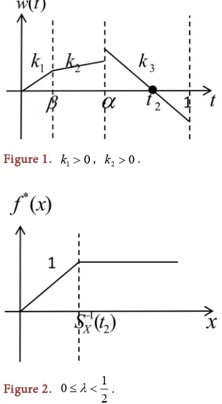
t is disconti-nuous at the point t=α. Therefore, we consider the followings.

1). When k1>0, there has three cases about k2, which are k2 >0, k2 =0 and k2 <0.

a) If k2 >0 , then

ψ α

( )

>0. t2 exists since

ψ α

( )

+ >

ψ α

( )

>0 and

( )

1 0

ψ

= − <

ρ

_{. Note that}

ψ

( )

t >0_in

( )

0,t₂ ,

ψ

( )

t <0_in

(

t₂,1

]

as Figure 1. With the expression (3.7), we have that _{h x}*

( )

₌₁_for

(

1

_{( )}

)

2 0, _X

x_∈ S t− _,

( )

* ₀

h x = _for

(

1

( )

)

2 ,

X

x_∈ S t− _∞ _{as Figure 2, thus} *

( )

1

( )

2

X

f x _{= ∧}x S t− _.

b) If k2 =0, then

ψ α

( )

>0. Similar to 1), f x*

( )

= ∧x S tX−1

( )

2 .

c) When k2 <0 ,

ψ α

( )

has three cases

ψ α

( )

>0 ,

ψ α

( )

=0 and

( )

0

ψ α

< _{. Since}

ψ

( )

t _{is discontinuous at the point}t=α_{, we have to}

con-sider the cases of

ψ α

( )

+ .

i) If

ψ α

( )

≥0_{, then}

ψ α

( )

+ >0_{. Therefore,} t₂ exists.

ψ

( )

t >0_in

( )

0,t₂ ,

( )

t 0

ψ

< in

(

t2,1

]

. Furthermore, h x*

( )

=1 for x∈

(

0,S tX−1

( )

2

)

, h x*

( )

=0

for

(

1

( )

)

2 ,

X

x_∈ S t− _∞ _{, so} *

( )

1

( )

2

X

f x _{= ∧}x S t− _.

ii) If

ψ α

( )

<0 , then t1 exists. If

ψ α

( )

+ >0 , then t2 exists since

( )

1 0

ψ

< . Note that

ψ

( )

t >0 in

( )

0,t1 and

(

α

+,t2

]

,

ψ

( )

t <0 in

(

t1,

α

]

and

(

t2,1

]

( )

=1 for x∈

(

0,SX−1

( )

t2

)



(

SX−1

( )

α ,SX−1

( )

t1

)

,

( )

* ₀

h x = _for

(

1

( )

1

( )

)

(

1

( )

)

2 , 1 ,

X X X

x_∈ S− t S− α _ S− t _∞ _{, so}

( )

(

( )

)

(

( )

)

* 1 1 1 1

2 1

X X X X

f x x S− t x S− α S− t S− α

+

= ∧ + − ∧ − .

iii) If

ψ α

( )

<0, then t1 exists. When

ψ α

( )

+ ≤0,

ψ

( )

t >0 in

( )

0,t1 ,

( )

t 0

ψ

< _in

(

t₁,1

]

. Furthermore, _{h x}*

( )

₌₁_for

(

1

_{( )}

)

1 0, _X

x_∈ S t− _, _{h x}*

( )

₌₀ for

(

1

( )

)

1 ,

X

x_∈ S− t _∞ _{, so} *

( )

1

( )

1

X

f x _{= ∧}x S t− _.

(9)

[image:9.595.294.453.77.366.2]

DOI: 10.4236/jmf.2019.91002 19 Journal of Mathematical Finance Figure 1. k1>0, k2>0.

Figure 2. 0 1 2

λ

≤ < _.

a) When

ψ α

( )

+ >0_{, we can derive that}

ψ

( )

t >0_in

(

α

,t₂

)

,

ψ

( )

t =0_in

[ ]

0,

β

, and

ψ

( )

t

<

0

in

(

β α

,

]

and

(

t

2

,1

]

( )

=1 for

( )

)

(

( )

)

1 1 1

2

0, X X , X

x _ S− t S− α S− β

∈   , _{h x}*

( )

₌₀_for

(

1

_{( )}

1

_{( )}

)

2 ,

X X

x_∈ S− t S− α _{, and}

( )

*

h x =ξ for 1

( )

_,

)

X

x_∈_S− β _∞

 . Therefore,

( )

(

( )

)

(

( )

)

(

( )

)

* 1 1 1 1 1

2

X X X X X

f x x S− t x S− α S− β S− α ξ x S− β

+ +

= ∧ + − ∧ − + − .

b) When

ψ α

( )

+ ≤0_,

ψ

( )

t =0_in

[ ]

0,

β

_and

ψ

( )

t <0_in

(

β

,1

]

_. Furthermore, _{h x}*

( )

₌₁_for _0, 1

_{( )}

)

X

x _ S− β

∈  , and _{h x}*

( )

₌_ξ _for

( )

)

1 _,

X

x_∈_S− β _∞

 . Therefore, f x*

( )

= ∧x SX−1

( )

β +ξ

(

x S− X−1

( )

β

)

₊.

3). When k1<0, note that k2 <0 and

ψ α

( )

<0. There has three cases for

( )

ψ α +

.

a) When

ψ α

( )

+ >0_,

ψ

( )

t >0_in

(

α

,t₂

)

_and

ψ

( )

t <0_{in other cases.} Furthermore, _{h x}*

( )

₌₁_for

(

1

_{( )}

)

(

1

_{( )}

)

2

0, _X _X ,

x_∈ S t− _ S− α _∞ _, _{h x}*

( )

₌₀ _for

( )

(

1 1

)

2 ,

X X

x_∈ S− t S− α _{. Therefore,} *

_{( )}

1

_{( )}

(

1

_{( )}

)

2

X X

f x x S− t x S− α

+

= ∧ + − _.

b) If

ψ α

( )

+ ≤0, then

ψ

( )

t <0 in

( )

0,1 . Therefore, _{h x}*

( )

₌₁_when

(

0,

)

x∈ ∞ , _{f x}*

( )

₌_x_. _ Theorem 4.3 For 1 1

2< ≤λ , and any ceded loss function

f x

( )

∈

F

, optimal

reinsurance contracts _f*_{to Problem}₁_{are given as follows}_: 1). If k1>0 and k2 ≥0, then f x*

( )

=

(

x S− X−1

( )

t2

)

₊.

(10)

( )

(

)

( )

(

)

(

( )

)

(

( )

)

( )

(

)

( )

1 2

* 1 1 1 1

2 2 1

1 1

, 0,

, 0, 0,

, 0, 0.

X

X X X X

X

x S t

f x x S t S S t x S t

x S t

ψ α

α ψ α ψ α

ψ α ψ α

− + − − − − + + − +  − ≥  

=_ − ∧ − + − < + >



− < + ≤



3). If k1=0, then

( )

(

( )

)

(

( )

)

(

( )

)

( )

(

)

( )

1 1 1 1

2 2

*

1

, 0,

, 0.

X X X X

X

x S t S S t x S

f x

x S

α ξ β ψ α

ξ β ψ α

− − − −

+ +

− +

 − ∧ − + − + >

 = 

− + ≤



4). If k1<0, then

( )

(

( )

)

(

( )

)

( )

1 1 1

2 2

* , 0,

0, 0.

X X X

x S t S S t

f x

α

ψ α

− − −

+

 − ∧ − + >

 = 

+ ≤ 

Proof. Analyse the optimal reinsurance contract with (3.9) for the case

1 ₁

2< ≤λ .

1). When k1>0, there has three cases about k2.

[image:10.595.192.537.72.259.2]

a) If k2 >0, then

ψ α >

( )

0

. Since

ψ α

( )

+ >

ψ α

( )

>

0

and

ψ

( )

1 = − <

ρ

0

, then t2 exists. Therefore,

ψ

( )

t

>

0

in

( )

0,

t

2 and

ψ

( )

t

<

0

in

(

t

2

,1

]

as Figure 1. With the expression (3.9), we have that _{h x}*

( )

₌₀ _for

( )

(

1

)

2 0, _X

x_∈ S t− _and _{h x}*

( )

₌₁ _for

(

1

_{( )}

)

2 ,

X

x_∈ S t− _∞ _{as Figure 3, so}

( )

(

( )

)

* 1

2

X

f x x S− t

+

= − .

b) If k2 =0, then

ψ α >

( )

0

. Similar to 1), f x*

( )

=

(

x S− X−1

( )

t2

)

₊.

c) When k2 <0 ,

ψ α

( )

has three cases

ψ α >

( )

0

,

ψ α =

( )

0

and

( )

0 ψ α <

. Since

ψ

( )

t

is discontinuous at the point t=α, we have to con-sider the cases of

ψ α +

( )

.

i) If

ψ α ≥

( )

0

, then

ψ α + >

( )

0

, t2 exists since

ψ

( )

1 = − <

ρ

0

. Note that

( )

t

0 ψ

>

in

( )

0,

t

2 and

ψ

( )

t

<

0

in

(

t

2

,1

]

( )

=0 for

( )

(

1

)

2 0, _X

x_∈ S t− _, _{h x}*

( )

₌₁_for

(

1

_{( )}

)

2 ,

X

x_∈ S t− _∞ _{, so} *

( )

(

1

( )

)

2

X

f x x S− t

+

= − .

ii) If

ψ α <

( )

0

and

ψ α + >

( )

0

, then t1 and t2 exists. Clearly

ψ

( )

t

>

0

in

( )

0,

t

1 and

(

α+

,

t

2

]

,

ψ

( )

t

<

0

in

(

t

1

,

α

]

and

(

t

2

,1

]

. Furthermore,

( )

* ₀

h x = for

(

1

( )

)

(

1

( )

1

( )

)

2 1

0, _X _X , _X

x_∈ S− t S− α S− t

 , _{h x}*

( )

₌₁_for

( )

(

1 1

)

(

1

( )

)

2 , 1 ,

X X X

x_∈ S− t S− α _ S− t _∞ _{, so}

( )

(

( )

)

(

( )

)

(

( )

)

* 1 1 1 1

2 2 1

X X X X

f x x S− t S− α S− t x S− t

+ +

= − ∧ − + − .

iii) If

ψ α <

( )

0

and

ψ α + ≤

( )

0

, then t1 exists. Clearly,

ψ

( )

t

>

0

in

( )

0,

t

1 and

ψ

( )

t

<

0

in

(

t

1

,1

]

( )

=0 for x∈

(

0,S tX−1

( )

1

)

,

( )

* ₁

h x = for

(

1

( )

)

1 ,

X

x_∈ S− t _∞ _{, so} *

( )

(

1

( )

)

1

X

f x x S− t

+

= − .

2). When k1=0, from (4.6) and (4.7), we obtain that k2 <0 and

ψ α <

( )

0

. Next, we consider the cases of

ψ α + >

( )

0

.

a) When

ψ α + >

( )

0

, we can derive that

ψ

( )

t

>

0

in

(

α

,

t

2

)

,

ψ

( )

t

=

0

in

[ ]

0,

β

, and

ψ

( )

t

<

0

_in

(

β α

,

]

and

(

t

2

,1

]

( )

=0 for

( )

)

(

( )

)

1 1 1

2

0, _X _X , _X

x _ S− t S− α S− β

∈   , _{h x}*

( )

₌₁_for

(

1

_{( )}

1

_{( )}

)

2 ,

X X

x_∈ S− t S− α _{, and}

( )

*

h x =ξ when 1

( )

_,

)

X

x_∈_S− β _∞

 . Therefore,

( )

(

( )

)

(

( )

)

(

( )

)

* 1 1 1 1

2 2

X X X X

f x x S− t S− α S− t ξ x S− β

+ +

(11)

b) When

ψ α

( )

+ ≤0,

ψ

( )

t =0 in

[ ]

0,

β

_and

ψ

( )

t <0 in

(

β

,1

]

. Fur-thermore, _{h x}*

( )

₌₀_for _0, 1

_{( )}

)

X

x _ S− β

∈  , and _{h x}*

( )

₌_ξ _for

( )

)

1 _,

X

x_∈_S− β _∞

 . Therefore, f x*

( )

=ξ

(

x S− X−1

( )

β

)

₊.

3). When k1<0, note that k2 <0 and

ψ α

( )

<0. There has three cases for

( )

ψ α

+ .

a) When

ψ α

( )

+ >0_,

ψ

( )

t >0_in

(

α

,t₂

)

and

ψ

( )

t <0_{in other cases.} Furthermore, _{h x}*

( )

₌₀ _for

(

1

_{( )}

)

(

1

_{( )}

)

2

0, X X ,

x_∈ S t− S− α _∞

 , _{h x}*

( )

₌₁ _for

( )

(

1 1

)

2 ,

X X

x_∈ S− t S− α _{. Therefore,} *

( )

(

1

( )

)

(

1

( )

1

( )

)

2 2

X X X

f x x S− t S− α S− t

+

= − ∧ − .

b) If

ψ α

( )

+ ≤0, then

ψ

( )

t <0 in

( )

0,1 . Therefore, _{h x}*

( )

₌₀_when

(

0,

)

x∈ ∞ _, _{f x}*

( )

₌₀_. _

Example 4.1. Similar to Example 2.1, we assume the risk is measured by the GlueVaR risk measures under the expectation premium principle, for

λ

∈

[ ]

0,1 _,

[ ]

0,1

ξ

∈ ,

ω

i∈

[ ]

0,1 , i=1,2,3 and ω ω1+ 2+ω3=1, optimal reinsurance con-tracts are given as follows.

From the reinsurer’s point of view, as Case 1 in Table 2, the optimal reinsur-ance strategy can be in form of limited quota-share, _{f x}*

( )

_{= ∧}_x _405.47_{, which} means that if initial loss X less than 405.47, the case that an insurer ceded all loss to a reinsurer is optimal, and if initial loss X more than 405.47, the case that an insurer ceded 405.47 to a reinsurer is optimal.

[image:11.595.296.451.417.568.2]

From the insurer’s point of view, as Case 6 in Table 2, the optimal reinsurance strategy _{f x}*

( )

₌₀_{, which means that an insurer should retain all loss to} achieve itself optimality.

Figure 3. 1 1 2< ≤λ .

Table 2. Optimal ceded loss function.

Case α β ω1 ω2 ω3 λ ρ ( )

*

f x

1 0.05 0.01 0.20 0.30 0.50 0.00 0.50 x∧405.47

2 0.10 0.05 0.10 0.05 0.85 0.20 1.00 x∧2995.73+ξ(x−2995.73)+

3 0.15 0.10 0.15 0.10 0.75 0.40 2.00 x∧1099.61+(x−1897.12)+

4 0.20 0.15 0.40 0.20 0.40 0.60 1.50 (x−916.29)+

5 0.25 0.20 0.50 0.20 0.30 0.80 2.00 (x−1099.61)+∧286.68+ξ(x−1609.44)+

[image:11.595.210.543.603.738.2]

(12)

From the perspectives of an insurer and a reinsurer, as Cases 2 - 5. Note that Cases 2 and 5 include the parameter

ξ ∈

[ ]

0,1

, which means that reinsurance contracts can be different forms when the loss risk has been minimized. Case 3 means that the stop-loss after quota-share reinsurance (which is to say a stop-loss will be applied after a quota-share reinsurance) is optimal. Case 4 means that stop-loss reinsurance is optimal.

5. Conclusion

This article has studied the optimal reciprocal reinsurance with the GlueVaR distortion risk measures under the expected value premium principle. The Glu-eVaR distortion risk measure is a linear combination of two TVaR and one VaR with different confidence levels, which adds the difficulty than the case of only one VaR or the case of only one TVaR when we derive the optimal reinsurance contract. In this paper, we have expressed GlueVaR as a linear combination of three distortion risk measures with different distortion functions. Therefore, we can use MIF formula to deal with the complex optimization problems easily. The results indicate that depending on the risk measures’s level of confidence (

α

and β_{), the safety loading (}ρ_{) for the reinsurance premium, weight (}λ_{) of an}

insurer in the reciprocal reinsurance model and the proportions (ω ω1, 2 and 3

ω _{) of the three risk measures in the definition of GlueVaR, the optimal}

rein-surance can be in the forms of quota-share, stop-loss, change-loss, or their com-bination, for example, stop-loss after quota-share. This paper has not considered the practical constraints, such as risk constraints or reinsurance premium con-straints, which can be studied at a later time.

Acknowledgements

The author would like to thank the anonymous referees for helpful comments and suggestions, which have led to significant improvements of the present pa-per.

Author Contributions

These authors contributed equally to this work.

Conflicts of Interest

The authors declare no conflict of interest.

Funding

The research was supported by the National Natural Science Foundation of China (No. 11171179, 11571198).

References

(13)

https://doi.org/10.2143/AST.37.1.2020800

[2] Cai, J., Tan, K.S., Weng, C. and Zhang, Y. (2008) Optimal Reinsurance under VaR and CTE Risk Measures. Insurance: Mathematics and Economics, 43, 185-196.

https://doi.org/10.1016/j.insmatheco.2008.05.011

[3] Cheung, K.C. (2010) Optimal Reinsurance Revisited: A Geometric Approach. Astin Bulletin, 40, 221-239. https://doi.org/10.2143/AST.40.1.2049226

[4] Chi, Y. and Tan, K.S. (2011) Optimal Reinsurance under VaR and CVaR Risk Measures: A Simplified Approach. Astin Bulletin, 41, 487-509.

[5] Chi, Y. and Tan, K.S. (2013) Optimal Reinsurance with General Premium Prin-ciples. Insurance: Mathematics and Economics, 52, 180-189.

[6] Li, P., Zhou, M. and Yin, C.C. (2015) Optimal Reinsurance with Both Proportional and Fixed Costs. Statistics and Probability Letters, 106, 134-141.

https://doi.org/10.1016/j.spl.2015.06.024

[7] Cai, J., Liu, H.Y. and Wang, R.D. (2017) Pareto-Optimal Reinsurance Arrangements under General Model Settings. Insurance: Mathematics and Economics, 77, 24-37.

[8] Chi, Y.C. and Meng, H. (2014) Optimal Reinsurance Arrangements in the Presence of Two Reinsurers. Scandinavian Actuarial Journal, 5, 424-438.

https://doi.org/10.1080/03461238.2012.723638

[9] Yin, C.C. (2018) Remarks on Equality of Two Distributions under Some Partial Orders. Acta Mathematicae Applicatae Sinica, English Series, 34, 274-280.

https://doi.org/10.1007/s10255-018-0744-z

[10] Yuen, K.C. and Yin, C.C. (2012) Asymptotic Results for Tail Probabilities of Sums of Dependent and Heavy-Tailed Random Variables. Chinese Annals of Mathemat-ics, Series B, 33B, 557-568. https://doi.org/10.1007/s11401-012-0723-2

[11] Yin, C.C. and Zhu, D. (2016) New Class of Distortion Risk Measure and Their Tail Asymptotics with Emphasis on VaR. Journal of Financial Risk Management, 7, 12-23. https://doi.org/10.4236/jfrm.2018.71002

[12] Zhu, D. and Yin, C.C. (2018) Two Sufficient Conditions for Convex Ordering on Risk Aggregation. Abstract and Applied Analysis, 2018, Article ID: 2937895.

https://doi.org/10.1155/2018/2937895

[13] Zhu, D. and Yin, C.C. (2018) Stochastic Optimal Control of Investment and Divi-dend Payment Model under Debt Control with Time-Inconsistency. Mathematical Problems in Engineering, 2018, Article ID: 7928953.

https://doi.org/10.1155/2018/7928953

[14] Zhu, Y.Z., Chi, Y.C. and Weng, C. (2014) Multivariate Reinsurance Designs for Mi-nimizing an Insurer’s Capital Requirement. Insurance: Mathematics and Econom-ics, 59, 144-155. https://doi.org/10.1016/j.insmatheco.2014.09.009

[15] Tan, K.S., Weng, C. and Zhang, Y. (2011) Optimality of General Reinsurance Con-tracts under CTE Risk Measure. Insurance: Mathematics and Economics, 49, 175-187. https://doi.org/10.1016/j.insmatheco.2011.03.002

[16] Cheung, K.C., Sung, K., Yam, S. and Yung, S. (2014) Optimal Reinsurance under General Law-Invariant Risk Measures. Scandinavian Actuarial Journal, 1, 72-91.

https://doi.org/10.1080/03461238.2011.636880

(14)

109-120.https://doi.org/10.1016/j.insmatheco.2014.08.010

[18] Cui, W., Yang, J.P. and Wu, L. (2013) Optimal Reinsurance Minimizing the Distor-tion Risk Measure under General Reinsurance Premium Principles. Insurance: Ma-thematics and Economics, 53, 74-85.

[19] Cheung, K.C. and Lo, A. (2017) Characterizations of Optimal Reinsurance Treaties: A Cost Benefit Approach. Scandinavian Actuarial Journal, 1, 1-28.

https://doi.org/10.1080/03461238.2015.1054303

[20] Assa, H. (2015) On Optimal Reinsurance Policy with Distortion Risk Measures and Premiums. Insurance: Mathematics and Economics, 61, 70-75.

[21] Zhuang, S.C., Weng, C., Tan, K.S. and Assa, H. (2016) Marginal Indemnification Function Formulation for Optimal Reinsurance. Insurance: Mathematics and Eco-nomics, 67, 65-76.https://doi.org/10.1016/j.insmatheco.2015.12.003

[22] Lo, A. (2017) A Neyman-Pearson Perspective on Optimal Reinsurance with Con-straints. Astin Bulletin, 47, 467-499.https://doi.org/10.1017/asb.2016.42

[23] Jiang, W.J., Hong, H.P. and Ren, J.D. (2017) On Pareto-Optimal Reinsurance with Constraints under Distortion Risk Measures. European Actuarial Journal, 8, 215-243.https://doi.org/10.1007/s13385-017-0163-1

[24] Belles-Sampera, J., Guillen, M. and Santolino, M. (2014) Beyond Value-at-Risk: GlueVaR Distortion Risk Measures. Risk Analysis, 34, 121-134.