ISSN Online: 2327-5227 ISSN Print: 2327-5219
DOI: 10.4236/jcc.2018.611007 Nov. 19, 2018 77 Journal of Computer and Communications
Analysis of Seasonal Characteristics of Thermal
Environment Based on Urban Sub-Pixel Land
Use Types
Jingyuan Cheng
1,2, Youshui Zhang
1,2*1Institute of Geography, Fujian Normal University, Fuzhou, China
2School of Geographical Science, Fujian Normal University, Fuzhou, China
Abstract
Seasonal variations will cause the differences in the distribution of urban thermal environment. Therefore, it is essential for analyzing the distribution of land surface temperature (LST) in different seasons under the same land use type. In this paper, fully constrained least squares method of linear spec-tral mixture analysis was used to extract the information of land cover frac-tion. According to the differences in the degree of the urban development, the study area is divided into three regions, for estimating the differences in the distribution of urban thermal environment. Ternary triangular charts were drawn to analyze the impact of each land use type on seasonal UHI. Contri-bution index (CI) of each land cover was calculated to analysis of the impact of each land use type on LST. The results of this study indicate that the ex-treme differences in temperature exex-tremes occur in summer, followed by spring, autumn, and winter. In the spring, high LST areas appear in industri-al, bare land; high LST areas in summer occur in the CBD, light industriindustri-al, and cover crops; the high LST areas in autumn appear in the CBD, high-density residential; in winter, the distribution of low-density and medium-density residential areas, crops and lawns will inhibit the urban heat island effect. The analytical methodologies that be used in this study can help to quantify urban thermal environmental functions effect of different land use type and explore the climate adaptation potential of cities.
Keywords
Land Surface Temperature, Linear Spectral Unmixing, Loop Zoning, Ternary Triangular Charts, Fuzhou Province
How to cite this paper: Cheng, J.Y. and Zhang, Y.S. (2018) Analysis of Seasonal Characteristics of Thermal Environment Based on Urban Sub-Pixel Land Use Types. Journal of Computer and Communications, 6, 77-90.
https://doi.org/10.4236/jcc.2018.611007
DOI: 10.4236/jcc.2018.611007 78 Journal of Computer and Communications
1. Introduction
As the basic physical quantity of energy balance in the geogas system, land Sur-face Temperature (LST) has considered to be one of the most important indica-tors for assessing of the urban thermal environment. The urban thermal envi-ronment obviously affect by seasonal variation. Long time series temperature data is often used to analyze daily, monthly, seasonal, and annual changes in ur-ban heat islands (HUI) [1]. Some indicators such as atmospheric circulation, cloudiness and aerosol are used to analyze the seasonal trends of UHI [2]. Com-pared with atmospheric temperature, spatial heterogeneity of LST existed strongly on urban scale [3] [4]. LST is more strongly influenced by Land-Use and Land-Cover Change (LULC) and human activities [5] [6]. What’s more, the impact of LULC on UHI is affected by seasonal variation [7] [8]. Clarification as to how changes in LULC contribute to observe variations in LST by seasonal changeable is necessary in order to reduce UHI impact and enable urban areas to adapt to climate change effectively.
Due to extreme urbanization, more and more nonurban land cover in urban space have been replaced by Impervious Surface Area (ISA) [9] [10]. The large impervious surface in urban will result in significant impacts in cities, including reduced evapotranspiration, increased surface runoff, increased storage and transfer of sensible heat, reduced air and water quality [11] [12]. However, the effects of urban development density on LST are not well understood. Therefore, this study focuses on the impact of urban development density within UHI in different region. According to urban overall planning of Fuzhou, the study area was divided into three region, internal city region, intercity region, and ru-ral-urban continuum.
In this paper, Fuzhou city was selected as the study area. Because 30 meter or lower resolution data (e.g. Landsat-class) are more suitable to map the extent and change of urban land cover [13] [14] [15], fully constrained least squares li-near spectral mixture analysis (LSMA) was used to obtain the sub-pixel LULC coverage information and the high-resolution image are used to verify the ex-tracted results by area comparison method. According to the density of urban development, the study area is divided into three regions. The percent of ISA in each region based on pixels was divided to generate several of ISA coverage cat-egories to analyze the relationship between LST and land cover patterns. Season-al UHI plaque area and LST boxplots were used to anSeason-alyze the impact of each region on UHI. Base on the vegetation-impervious-soil (VIS) model, ternary triangular chart method was applied for LST for each season to analyze the im-pact of each season on UHI [16].
2. Study Area and Data
2.1. The Study Region
ex-DOI: 10.4236/jcc.2018.611007 79 Journal of Computer and Communications pansion of the city and the rapid increase of the impervious surface, local high LST areas appear in the city, and the UHI effect is serious. Therefore, choosing Fuzhou as a research area has typical significance. According to the “Urban overall planning of Fuzhou (2011-2020)” [19], minimum enclosing rectangle in the central city was selected as the research area. Combined with urban space structure planning in Fuzhou [20], the research area was divided into three re-gion, internal city rere-gion, intercity rere-gion, and rural-urban continuum in Figure 1.
2.2. Data and Preprocessing
In order to reflect the seasonal characteristics of UHI, the mid-season date of Landsat-8 images were selected to represent the spring, summer, autumn and winter. Because Fuzhou belongs to the subtropical marine monsoon climate, it’s difficult to obtain seasonal images in the same year in Cloud-prone and Raining Area. Therefore, bi-temporal Landsat-8 images (path 89/row 84) acquired on April 17, 2014, July 27, 2016, October 23, 2013 and December 13, 2014. The Google Earth image (acquired on October 1, 2013, April 11, 2014, December 18, 2014 and July 27, 2016) with 1 m spatial resolution were used as ancillary data for the assessment of the accuracy of sub-pixel LULC coverage information.
[image:3.595.284.461.490.683.2]All data used in this study were projected to the Universal Transverse Merca-tor (UTM) based on the high-resolution images of the same phase. The RMSE of the projection was <0.5 pixels. For Landsat images, Second Simulation of the Sa-tellite Signal in the Solar Spectrum (6S) and MODTRAN tools were used for ra-diometric calibration and atmospheric correction. In order to eliminate the in-fluence of waters in the study area on the spectral analysis of low reflectivity fea-tures, modified normalized difference water index (MNDWI) was calculated to extract water [21].
DOI: 10.4236/jcc.2018.611007 80 Journal of Computer and Communications
3. Methods
The methodology for this study consists of four steps. Step 1 includes retrieval of LST and fractional covers retrieval using LSMA. Step 2 includes accuracy as-sessment of sub-pixel LULC covers by area comparison method. Step 3 divides the fractional values of ISA base on the density of urban development and ana-lyzes the differences in the effects of each LULC on the LST of the four seasons with ternary triangular chart method and contribution rate. Step 4 according to the urban overall planning, divides the study area into three regions and analyze the seasonal spatial distribution of thermal environment in each annular region.
3.1. Spectral Unmixing and Accuracy Assessment
In this paper, the spectrum of pure pixels in the study area is unknown. There-fore, minimum noise fraction rotation (MNF) and pixel purity index (PPI) used to extracting the spectrum of pure pixels in the study area and regards
1 1
N i i= f =
∑
and fi ≥0 (fi the fraction of end-member i within the pixel)ascon-straint condition. The fully constrained least squares of LSMA used to extract fractional LULC values from OLI imagery (Formula 1). The advantage over un-constrained methods is that: 1) data segmentation and root mean square (RMS)calculated for each loop computing; 2) not calculate mask pixels with all band values of 0 [22].
, 1
N
b i i b b
i
R f R e
=
=
∑
+ (1)where Rb is spectral reflectance in band b; N is the number of end-members; fi
the fraction of end member i within the pixel; Ri b, the reflectance of end
mem-ber b in band i; eb is the residual error for band i.
Accuracy assessment of sub-pixel fractional covers by site investigation is time-consuming and laborious. Using the high-resolution image to extract frac-tional covers information, not only can obtain the higher precision than the low-resolution image extraction results, but also can be used as the validation of accuracy of the lower-resolution image .Six test sites within the study area about 2 km2 were selected for the accuracy estimation of fractional covers. The
ob-ject-oriented classification method and the artificial visual interpretation were used to extract the LULC information of the preprocessing high-resolution im-ages (the acquisition time is close to the Landsat image).Calculate the area of the Lands at image using (Formula (2)) and Mean Error (ME) between the Landsat and Google Earth images(Formula (3)).
2 1
n
OLI i i g
S =
∑
= f R (2)where SOLI is Landsat images’ fractional covers area; Rg is Landsat image’s
spatial resolution; n is test site’s total pixel numbers.
( OLI Google) / Google
ME= S −S S (3)
DOI: 10.4236/jcc.2018.611007 81 Journal of Computer and Communications
3.2. Landsat Surface Emissivity Calculation and LST Retrieval
The Landsat 8 TIRS includes two thermal infrared bands. Since the band 10 is located in the lower atmospheric absorption are aand band 11 has larger uncer-tainty data as USGS said, so the band 10 is more suitable for single-band’s LST Retrieval calculation [23] [24]. Convert the digital numbers of thermal bands to top of atmosphere (TOA) radiance using:L cal L
Lλ =M Q +A (4) where Lλ is the TOA radiance image of the thermal band; ML is the
band-specific multiplicative rescaling factor and AL is the band-specific additive
rescaling factor; QCAL is the pixel digital number for thermal band 10.
There are many LST retrieval algorithms for Landsat images. The mono-window algorithm improved by Jimenezmunoz and Sobrino which requires less atmos-pheric correction parameters and has higher precision is widely used in Landsat TIRS LST retrieval. [25] (Formula (5)).
1
1 2 3
[ ( ) ]
LST=γ ε− ⋅ψ Lλ+ψ +ψ +δ (5)
where ε is surface emissivity; γ and δ are the estimated parameters from the li-near formula of Planck’s law; ψ1, ψ2 and ψ3 are three functions gained from actual atmospheric parameters (Formulas (6)-(8)).
1 1
ψ τ
= (6)
2 L L
ψ
τ
↑ ↓
= − − (7)
3 L
ψ = ↓ (8) where τ is atmospheric transmission; L↑ and L↓ are up welling and down
welling radiance.
3.3. Contributions of the Landscape Pattern to the Urban Thermal
Environment
Due to the range of LST is inconsistent in different season, it is impossible to di-rectly compare the inversion results of the four seasons’ LST. In this paper, con-tribution index (CI) was used to analyze the difference in the average LST be-tween each fractional covers area in different urban development region and en-tire study area (Formula (9)). CI estimates the contribution of landscape pattern in each urban development region to the LST dynamic increase or decrease, and it is based on spatial and temporal dimensions to analyze the contribution of each fractional category to urban heat island effect.
/
i dif i sum
CI =LST ⋅S S (9)
where CIi is the contribution of the each fractional category to the regional LST; LSTdif· is the average LST difference between the each fractional category region
and the entire area; Si is the area of fractional category region; Ssum is the area of
DOI: 10.4236/jcc.2018.611007 82 Journal of Computer and Communications
3.4. Normalized LST Values
As the season changes, it will affect the relative strength of the surface tempera-ture. In this paper, LST normalized was used to unify the LST distribution range from 0 to 1 without changing the spatial distribution characteristics of the ther-mal environment (Formula (10)).
min max min
( i ) / ( )
i s s S s
N = T −T T −T (10)
where TSi is LST for a given pixel; TSmin and Tsmax is the minimum and
maximum LST value in an image.
4. Results and Discussion
4.1. Accuracy Analysis of the Sub-Pixel Fractional Covers
The fully constrained least squares of LSMA was used to unmix mixed pixel, and V-I-S model was used to define categories of end members [16]. Wherein, the category with high reflectivity and low reflectivity are superimposed and summed to represent the coverage value of the ISA. Figure 2 shows the each end member fractions covers in the study.
[image:6.595.210.538.551.743.2]According to the result, the spring average RMS is 0.0008, the summer aver-age is RMS 0.0011, the autumn averaver-age RMS is 0.0016, and the winter averaver-age RMS is 0.0006, which is less than the required 0.02 accuracy requirement [22]. To further verify the LULC extraction results, each fractional covers category was extracted from Google Earth images, which was used to assess the accuracy of the fractional covers estimate from Landsat. Six test sites were chosen in Fig-ure 2(1a) for the accuracy analysis. ME (Formula (4)) was calculated to analyze the difference of each fractional cover extraction result from two types of images. Table 1 shows the results of the accuracy assessment of LSMA. The area of frac-tional covers in the six test sites showed only small differences, which explained that the number of end members in this study is appropriate, and the fractional covers extraction results are reliable.
Table 1.Statistical table of average error of land use type extraction results (%).
site spring summer autumn winter
ISA VEG SOIL ISA VEG SOIL ISA VEG SOIL ISA VEG SOIL 1 −9.02 5.34 6.44 9.57 −8.56 −7.13 5.50 1.83 −3.56 7.80 −8.26 2.01 2 8.31 8.47 2.81 1.58 −6.38 2.73 7.28 −7.62 −0.05 −5.75 −2.66 9.81
3 3.39 −7.12 8.86 −6.44 9.50 5.80 −2.05 3.41 −1.34 −6.74 −2.74 −3.75
4 −6.47 −8.03 −6.59 −1.16 −4.40 9.22 −3.16 9.20 4.25 −5.92 6.42 9.88
5 −2.29 9.27 −5.93 −4.49 −3.68 −6.48 −7.13 0.22 9.06 −0.19 9.29 7.69
6 2.27 2.62 8.20 9.25 −4.10 −8.02 5.74 −4.94 6.66 6.49 −5.38 −2.45
DOI: 10.4236/jcc.2018.611007 83 Journal of Computer and Communications Figure 2. Fractional images by LSMA (a, b, c represent Fractional impervious surface, the soil and vegetation, 1, 2, 3, 4 represent spring, summer, autumn, winter, and the red sites in 1a represent test sites used for accuracy assessment).
4.2. Urban Thermal Intensity Analysis on Season Variations
4.2.1. Influence of Sub-Pixel LULC on Seasonal LST
The “Formulas (4)-(8)” were used to retrieve the LST of the four seasons in the study area. Figure 3 shows the results of seasonal LST retrieval.
DOI: 10.4236/jcc.2018.611007 84 Journal of Computer and Communications Figure 3. The spatial distribution of surface temperature in the four seasons. (a) Spring; (b) Summer; (c) Autumn; (d) Winter.
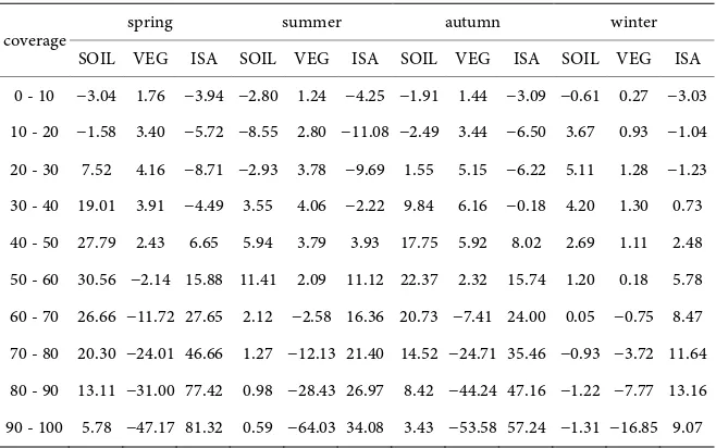
Table 2. The seasonal contribution rate of land use types at all levels to the surface temperature (%).
coverage spring summer autumn winter
SOIL VEG ISA SOIL VEG ISA SOIL VEG ISA SOIL VEG ISA 0 - 10 −3.04 1.76 −3.94 −2.80 1.24 −4.25 −1.91 1.44 −3.09 −0.61 0.27 −3.03 10 - 20 −1.58 3.40 −5.72 −8.55 2.80 −11.08 −2.49 3.44 −6.50 3.67 0.93 −1.04 20 - 30 7.52 4.16 −8.71 −2.93 3.78 −9.69 1.55 5.15 −6.22 5.11 1.28 −1.23 30 - 40 19.01 3.91 −4.49 3.55 4.06 −2.22 9.84 6.16 −0.18 4.20 1.30 0.73 40 - 50 27.79 2.43 6.65 5.94 3.79 3.93 17.75 5.92 8.02 2.69 1.11 2.48 50 - 60 30.56 −2.14 15.88 11.41 2.09 11.12 22.37 2.32 15.74 1.20 0.18 5.78 60 - 70 26.66 −11.72 27.65 2.12 −2.58 16.36 20.73 −7.41 24.00 0.05 −0.75 8.47 70 - 80 20.30 −24.01 46.66 1.27 −12.13 21.40 14.52 −24.71 35.46 −0.93 −3.72 11.64 80 - 90 13.11 −31.00 77.42 0.98 −28.43 26.97 8.42 −44.24 47.16 −1.22 −7.77 13.16 90 - 100 5.78 −47.17 81.32 0.59 −64.03 34.08 3.43 −53.58 57.24 −1.31 −16.85 9.07
In Table 2, the positive contribution rate indicates that the fractional covers in this interval promote the increase of urban thermal environment in the current season; the negative contribution rate indicates a reduction of urban thermal en-vironment in promotion; the absolute value of the contribution rate indicates the influence of the coverage categories on the thermal environment in the current season.
[image:8.595.210.539.292.498.2]DOI: 10.4236/jcc.2018.611007 85 Journal of Computer and Communications Since the contribution rate can only analyze the degree of influence of a single type of fractional covers on the LST. In this paper, according to the V-I-S model in Figure 4, the LULC in the pixel was defined by proportion of three types of fractional covers in mixed pixels. And an LST variable was added to the V-I-S model to analyze the impact of each fractional cover on urban thermal environ-ment in the four seasons in Figure 5.
[image:9.595.255.492.337.551.2]In Figure 5, the red map indicates that this pattern of LULC promotes the urban LST increase; the blue map represents the pattern of LULC reduce the seasonal LST. Combined with the definition of V-I-S model can be found, in the spring, high LST areas appear in industrial, bare land and desert, with no ob-vious low LST areas; High LST areas in summer occur in the CBD, light indus-trial, and covercrops, and low LST areas appear in low-density residential and forest; the high LST areas in autumn appear in the CBD, high-density residential and range land, and the low LST areas appear in cover crops and lawn areas; in winter, light industry and heavy industry are the main areas of high LST distri-bution, the distribution of low-density and medium-density residential areas, crops and lawns will inhibit the urban heat island effect.
Figure 4. Illustration map of V-I-S (vegetation-impervious surface -soil) model.
[image:9.595.63.537.583.694.2]DOI: 10.4236/jcc.2018.611007 86 Journal of Computer and Communications
4.2.2. The Influence of Urban Development on Seasonal Thermal Environment
According to the “Urban overall planning of Fuzhou (2011-2020)”, the study area was divided into three regions, internal city region, intercity region, and rural-urban continuum. Boxplot is a method of depicting numerical data sets by quartile graphics. In this paper, boxplot was used to analyze the distribution of seasonal urban thermal environment base three regions in Figure 6. It can be seen from Figure 6 that the LST extremes of the intercity region differ greatly, followed by the rural-urban continuum and the interior of the city is smaller. With the season change, the maximum temperature difference between the var-ious surface areas is the largest in summer, followed by spring and autumn, and the smallest in winter. Through the analysis of the mean and median LST of each region, it can find that the distribution of intercity region’s LST is more dis-persed, followed by the rural-urban continuum, and the distribution of internal city region’s LST is more concentrated. The concentration is from high to low in winter and autumn, spring, summer.
[image:10.595.58.541.538.737.2]Due to seasonal variation, it is hard to directly analyze the difference of ther-mal environment in each season by using LST. Therefore, in this paper, formula 10was used to normalize the LST of the four seasons, and use the density seg-mentation technology to classify the images. According to the order from weak to strong of the UHI, The thermal environment of the study area is divided into seven levels: extremely low LST region (ETL), low LST region (LT), sub-low LST region (SLT), medium LST region (MT), sub-high LST region (SHT), high LST region (HT) and extremely high LST region (EHT). According to previous search, the three levels of sub-high LST, high LST and extremely high LST re-gion are the main plaques that constitute UHI [26]. To analyze the spatial varia-tion characteristics of four seasonal thermal environments in different urban development areas, the proportion of each LST level’s plaque in three regions was calculated (Table 3).
Table 3. Area of each LST level in every developing region (%).
site spring summer autumn winter
internal intercity rural-urban internal intercity rural-urban internal intercity rural-urban internal intercity rural-urban
ELT 0.72 1.11 2.84 0.01 0.05 1.14 0.24 0.78 3.75 0.29 2.76 7.09
LT 2.66 7.36 11.67 0.72 2.54 8.98 0.90 6.14 13.57 0.55 7.61 12.68
SLT 3.22 18.59 25.66 3.33 17.74 30.35 2.31 14.70 21.30 1.26 12.42 16.63
MT 11.12 32.73 35.31 8.09 38.24 39.95 10.13 34.74 35.04 9.02 26.63 32.98
SHT 13.86 12.22 10.88 5.62 10.02 8.38 16.17 16.47 12.81 16.70 18.47 19.35
HT 24.22 11.57 7.34 11.28 10.90 5.77 29.70 14.69 7.84 34.46 18.59 8.37
EHT 44.20 16.42 6.29 70.95 20.51 5.43 40.54 12.49 5.69 37.72 13.52 2.90
DOI: 10.4236/jcc.2018.611007 87 Journal of Computer and Communications Figure 6. The boxplot of the four seasons surface temperature.
Table 3 shows that the proportion of the UHI plaques in four seasons was not much changed. However, in the case of extremely high LST region, the area of internal city region in summer is the highest, and the lowest in winter; the inter-city region in summer is highest, the lowest in autumn; the rural-urban conti-nuum in spring is highest, and the lowest in winter. Combined with Figure 2, it can be found that the main LULC in internal city region is ISA; Most of the in-tercity region are impervious, and combined with the soil and vegetation; ru-ral-urban continuum is most covered by soil and vegetable. Therefore, Tab.3 can also be used for verification the impact of each fractional cover on urban thermal environment in the four seasons.
5. Conclusions
Seasonal variation will have a certain impact on urban thermal environment when urban LULC are similar. In this paper, the study was divided into three re-gion, internal city rere-gion, intercity rere-gion, and rural-urban continuum, accord-ing to urban overall plannaccord-ing of Fuzhou. Statistics of the four-season LST’s box-plots of three regions, which was used to analyze the distribution of seasonal ur-ban thermal environment base different development. Combined with the LST normalization results, the ratio of the seven LST levels areas in each developing region was counted to analyze the spatial variation characteristics of seasonal thermal environment in city. According to the fractional covers obtained by the LSMA, the research area was quantitatively partitioned into 10 levels. Base on the 10 regions, the contribution rate of each fractional cover seasonal LST is calculated. Combined with the ternary triangular charts, contribution rate was used to analysis of the combined effects of three types of land use on LST.
DOI: 10.4236/jcc.2018.611007 88 Journal of Computer and Communications 1) Seasonal contribution rate of each region can effectively analyze the impact of LULC on seasonal LST. It was found that when the density of the ISA in the pixel is greater than 40%, it will promote the urban thermal environment. The intensity of the four seasons is: spring > autumn > summer > winter; when the density of the vegetation is greater than 60%, it will reduce the urban thermal environment. The intensity of the four seasons is: summer > autumn > spring > winter; the effect of soil coverage on the thermal environment is greatly affected by the season, and the effects in spring and autumn are relatively close;
2) Ternary triangular charts can used to analysis of the combined effects of three types of land use on LST. It was found that in the spring, high LST areas appear in industrial, bare land; high LST areas in summer occur in the CBD, light industrial, and cover crops; the high LST areas in autumn appear in the CBD, high-density residential; in winter, the distribution of low-density and medium-density residential areas, crops and lawns will inhibit the urban heat island effect;
Based on the degree of development, the difference in the area of seasonal UHI plaques in different regions is not obvious. However, there is a difference in LST distribution: the LST extremes of the intercity region differ greatly, followed by the rural-urban continuum and the interior of the city is smaller. With the season change, the extreme LST in summer is largest, followed by spring and autumn, and the smallest in winter; the distribution of intercity region’s LST is more dispersed, followed by the rural-urban continuum, and the distribution of internal city region’s LST is more concentrated. The concentration is from high to low in winter and autumn, spring, summer.
Fund
Project supported by the Natural Science Foundation of Fujian Province, China (2018J01739) and Special Scientific Research Fund of Research Institutes Public Welfare Profession of Fujian Province, China (2019R1102).
Conflicts of Interest
The authors declare no conflicts of interest regarding the publication of this pa-per.
References
[1] Santamouris, M. (2014) On the Energy Impact of Urban Heat Island and Global Warming on Buildings. Energy & Buildings, 82, 100-113.
https://doi.org/10.1016/j.enbuild.2014.07.022
[2] Yeşilırmak, E. (2013). Temporal Changes of Warm-Season Pan Evaporation in a Semi-Arid Basin in Western Turkey. Stochastic Environmental Research & Risk Assessment, 27, 311-321. https://doi.org/10.1007/s00477-012-0605-x
DOI: 10.4236/jcc.2018.611007 89 Journal of Computer and Communications [4] Li, J., Ren, G., Ren, Y. and Zhang, L. (2014) Effect of Data Homogenization on
Es-timate of Temperature Trend and Urban Bias at Shenyang Station. 37, 297-303. [5] Liu, D., Yan, L.I. and Kong, F. (2013) Spatial Distribution of Land Surface
Temper-ature in Central City Proper and the Cooling of Objects Effect: A Case Study of Nanjing. Remote Sensing for Land & Resources, 25, 117-122.
[6] Nsubuga, F.W.N., Botai, J.O., Olwoch, J.M., Rautenbach, C.J.D., Kalumba, A.M., Tsela, P., et al. (2015) Detecting Changes in Surface Water Area of Lake Kyoga Sub-Basin Using Remotely Sensed Imagery in a Changing Climate. Theoretical & Applied Climatology, 127, 1-11.
[7] Han, F., Zhang, B.P., Zhao, F., Guo, B. and Liang, T. (2018) Estimation of Mass Elevation Effect and Its Annual Variation Based on Modis and NecpData in the Ti-betan Plateau. Journal of Mountain Science, 15, 1510-1519.
https://doi.org/10.1007/s11629-018-4865-x
[8] Liang, B.P., Ma, Y.F. and Hui, L.I. (2015) Research on Cooling Effect of the Land-scape Green Space and Urban Water in Guilin City. Ecology & Environmental Sciences.
[9] Arnold Jr., C.L. and Gibbons, C.J. (1996) Impervious Surface Coverage: The Emer-gence of a Key Environmental Indicator. Journal of the American Planning Associ-ation, 62, 243-258. https://doi.org/10.1080/01944369608975688
[10] Wilson, J.S., Clay, M., Martin, E., Stuckey, D. and Vedder-Risch, K. (2003) Evaluat-ing Environmental Influences of ZonEvaluat-ing in Urban Ecosystems with Remote Sens-ing. Remote Sensing of Environment, 86, 303-321.
https://doi.org/10.1016/S0034-4257(03)00084-1
[11] Ibrahim, G.F. (2017) Urban Land Use Land Cover Changes and Their Effect on Land Surface Temperature: Case Study Using Dohuk City in the Kurdistan Region of Iraq. 5, 13.
[12] Pal, S. and Ziaul, S. (2016) Detection of Land Use and Land Cover Change and Land Surface Temperature in English Bazar Urban Centre. Egyptian Journal of Remote Sensing & Space Science, 20. https://doi.org/10.1016/j.ejrs.2016.11.003
[13] Chen, X., Sun, H., Yang, H. and Zhang, Z. (2010) Urban Spatial Growth Analysis from Satellite-Derived Imperviousness in an Oasis City. International Conference on Environmental Science and Information Application Technology, 1, 517-520. [14] Frazier, A.E. and Wang, L. (2011) Characterizing Spatial Patterns of Invasive
Spe-cies Using Sub-Pixel Classifications. Remote Sensing of Environment, 115, 1997-2007. https://doi.org/10.1016/j.rse.2011.04.002
[15] Weng, Q. (2012) Remote Sensing of Impervious Surfaces in the Urban Areas: Re-quirements, Methods, and Trends. Remote Sensing of Environment, 117, 34-49. https://doi.org/10.1016/j.rse.2011.02.030
[16] Ridd, M.K. (1995) Exploring a V-I-S (Vegetation-Impervious Surface-Soil) Model for Urban Ecosystem Analysis through Remote Sensing: Comparative Anatomy for Citiesâ. International Journal of Remote Sensing, 16, 2165-2185.
https://doi.org/10.1080/01431169508954549
[17] Fuzhou City Bureau of Statistics. 2000 Fuzhou Statistical Yearbook. http://tjj.fuzhou.gov.cn/zz/fztjnj/2000fztjnj/#conTar
[18] Fuzhou City Bureau of Statistics. 2016 Fuzhou Statistical Yearbook. http://tjj.fuzhou.gov.cn/zz/fztjnj/2016fztjnj/#conTar
DOI: 10.4236/jcc.2018.611007 90 Journal of Computer and Communications [20] Fuzhou City Master Plan (2011-2020) Urban Area Spatial Structure.
http://ghj.fuzhou.gov.cn/zz/cxgh/ztgh_9041/200910/t20091018_431760.htm [21] Xu, H.Q. (2005) A Study on Information Extraction of Water Body with the
Mod-ified Normalized Difference Water Index (MNDWI). Journal of Remote Sensing, 9, 589-595.
[22] Myint, S.W., Brazel, A., Okin, G. and Buyantuyev, A. (2010) Combined Effects of Impervious Surface and Vegetation Cover on Air Temperature Variations in a Ra-pidly Expanding Desert City. Mapping Sciences & Remote Sensing, 47, 301-320. [23] Jiménez-Muñoz, J.C., Sobrino, J.A., Skoković, D., Mattar, C. and Cristóbal, J. (2014)
Land Surface Temperature Retrieval Methods from Landsat-8 Thermal Infrared Sensor Data. IEEE Geoscience & Remote Sensing Letters, 11, 1840-1843.
https://doi.org/10.1109/LGRS.2014.2312032
[24] Coll, C., Caselles, V., Valor, E. and Niclòs, R. (2012) Comparison between Different Sources of Atmospheric Profiles for Land Surface Temperature Retrieval from Sin-gle Channel Thermal Infrared Data. Remote Sensing of Environment, 117, 199-210. https://doi.org/10.1016/j.rse.2011.09.018
[25] Jimenezmunoz, J.C., Cristobal, J., Sobrino, J.A., Soria, G., Ninyerola, M., Pons, X., et al. (2008) Revision of the Single-Channel Algorithm for Land Surface Temperature Retrieval from Landsat Thermal-Infrared Data. IEEE Transactions on Geoscience & Remote Sensing, 47, 339-349. https://doi.org/10.1109/TGRS.2008.2007125