Visualising software as a particle system

Visualising Software as a Particle System

Simon Scarle

Computer Science & Creative Technologies University of the West of England

Bristol, BS16 1QY Email: simon.scarle@uwe.ac.uk

Neil Walkinshaw

The University of Leicester Leicester, LE1 7RH Email: nw91@le.ac.uk

Abstract—Current metrics-based approaches to visualise un-familiar software systems face two key limitations: (1) They are limited in terms of the number of dimensions that can be projected, and (2) they use fixed layout algorithms where the resulting positions of entities can be vulnerable to mis-interpretation. In this paper we show how computer games technology can be used to address these problems. We present the PhysVis software exploration system, where software metrics can be variably mapped to parameters of a physical model and displayed via a particle system. Entities can be imbued with attributes such as mass, gravity, and (for relationships) strength or springiness, alongside traditional attributes such as position, colour and size. The resulting visualisation is a dynamic scene; the relative positions of entities are not determined by a fixed layout algorithm, but by intuitive physical notions such as gravity, mass, and drag. The implementation is openly available, and we evaluate it on a selection of visualisation tasks for two openly-available software systems.

I. INTRODUCTION

Software visualisation is broadly concerned with the chal-lenge of representing software systems, which are notoriously intangible [1], in graphical terms that provide insight to a developer. A plethora of techniques have been developed [2], which can visualise various facets of a software system (e.g. metrics, or code clones) at different levels of abstraction (from individual lines up to architectural components). To facilitate comprehension to the user, many techniques adopt metaphors, such as cities [3], Minecraft worlds [4], or solar systems [5]. Existing approaches are ultimately restricted in terms of the range of dimensions by which they visualize software entities and their interrelationships. Entities are projected to Cartesian coordinates (x, y in 2D orx, y, z in 3D), and their attributes tend to be visualised in terms of space (e.g. the height of a building or volume of a cell in a Tree map), or colour (e.g. using a colour-scale from green to red to represent complexity). Relationships between entities are commonly visualised simply in terms of connecting lines or in terms of their relative proximity (sharing a neighbourhood in a city) – a feature that can lead to misinterpretation if two objects happen to be close to each other without a corresponding relationship. In this paper we introduce PhysViz - a software visualisation system that is built with a Computer Games framework, and takes advantage of several games technologies. PhysViz is based on the idea of attributing physical properties to software entities and relationships, thus increasing the dimensions in

which software can be represented. As with existing tech-niques, PhysViz provides the means by which to represent entities in terms of their spacial coordinates, proximity, and visual properties such as colour, size and transparency. How-ever, PhysViz also incorporates a basic implementation of Newtonian point-mass physics (a standard component of a games particle effects systems), which enables us to model entities in terms of physical attributes, such as their mass, action of drag or gravitational acceleration. These enable us to consider relationships in terms such as interactions of these forces. The resulting scene is therefore not (necessarily) static; depending on the configuration, entities (or groups thereof) can continuously interact with each other (e.g. by gravitational pull). These forces can convey characteristics that would not necessarily be apparent in a conventional visualisation, and can indeed be highlighted by motion on top of location.

The key contributions are as follows:

• A physical framework for software visualisation.

• An openly available implementation (PhysViz).

• Three visualisation case studies on two openly available systems. These visualisations re-interpret existing 2D static visualisations (Hot spot views, Inheritance (System Complexity), and Call Graphs) in a physical setting, and explore the additional information that physical properties can convey about a software system.

The case studies illustrate two of the key attractions of PhysViz (or the use of games-physics to visualise software in general). Firstly, a variety of different aspects of a software system can be visualised and explored. However, whereas existing visualisations rely on specific layout algorithms, the layout of the elements in PhysViz is ultimately determined by the same rules of Newtonian point-mass physics. Secondly, there is continuous visual feedback to the user. There is no need to wait for a layout to be rendered; the software system can be explored while the layout is taking shape.

JEdit and Weka. Finally, section VII presents conclusions and discusses our future work.

II. MOTIVATION

The task of understanding a software system and detecting problems within it can be daunting. Software systems are large, complex, and have possibly evolved over years (even decades), with contributions from many different developers. An unfamiliar developer who is tasked with the job of re-engineering such a system has to rapidly acquaint themselves with the core components of the system, their interrelation-ships, and any apparent problematic aspects [6].

In the early stages, a developer who is orientating them-selves in the system will not necessarily be certain of what they are looking for. They might be searching for beacons by which to orientate themselves for future comprehension tasks [7]. However, they will also want to flag up any indicators of poor “software quality” – a term that has notoriously evaded a concrete definition because it means different things to different people [8].

To address this problem approaches such as Polymetric Views [9] have been developed. These aim to present a large amount of (relevant) information about the system (i.e. struc-tural elements and associations, combined with their relevant metrics) in a succinct visualisation, which can be customised by the developer to highlight particular facets.

Such approaches present a useful solution to the aforemen-tioned problems. They have inspired a plethora of subsequent visualisations (c.f. Code City [3]). They attenuate the problem of information overload. They also encourage (albeit to a limited degree) exploration by the developer, by enabling them to change the parameters of the visualisation. Nevertheless, there remain two important (and closely related) limitations:

1) Conventional visualisations remain limited to a relatively small number of dimensions: On the face of it, there seem to be plenty of possible dimensions within a standard visualiza-tion upon which to project a software system. The relative locations of objects can be used to imply relationships such as mutual relevance, either in 2D [9], or 3D [10]. Software attributes (e.g. metrics) can be overlaid onto these locations by varying standard rendering parameters such as colour, geometry, line-thickness, opacity, etc. So location (x, y, z) and colour with transparency (r, g, b, α) alone represent 7 dimensions. If we add typical additional visual attributes such as shape and size, then a mere three-dimensional scatter plot presents 12 ways in which to vary the appearance of an element (or group of elements).

This can certainly be sufficient, especially when the de-veloper already has a reasonably well-formed idea of what they are looking for. There are well-established approaches such as Goal-Question-Metric [11] that can be used to align the ‘question’ to be answered about the software system with the metrics that can be visualised to answer it. Indeed, most visualisation approaches implicitly assume that the selection of metrics is underpinned by such a process [12].

In practice however, this assumption is not necessarily practical. A “goal” might be very non-specific, and its metrics might accordingly be difficult to identify. This is especially the case for exploratory tasks – e.g. when the goal is simply to assess the state of the system, and in doing so pick up on any key design features or potential flaws (c.f. “Read all the code in one hour” [6]). In such cases the huge range of different types of entities, relationships, and metrics by which to interpret them cannot be reduced to a specific ‘ideal’ combination.

2) There is a trade-off between the number of dimen-sions visualised and readability of the resulting scene: If we acquiesce in the need to visualise a larger number of dimensions, this has immediate consequences on readability and comprehensibility [13]. Even relatively sophisticated 3-D visualisations such as CodeCity [3] are only able to visualise three metrics at a time (though they do so very effectively). Thus an important question for us is: How can we effectively accommodate a larger number of dimensions, whilst maintain-ing the ease of interpretation for the developer?

III. GAMESENGINES– ASSETPIPELINES ANDPARTICLE

SYSTEMS

This paper is based on the observation that computer game technology can potentially provide a solution to the above problems. Computer games are similarly faced with the chal-lenge of presenting a huge amount of information (a typical computer game scene can contain hundreds or thousands of characters and objects). It is crucial for game-play that the game scene is computationally efficient to render – that it does not make unrealistic demands on computational resources and does not induce lag.

Modern games engines such as Unity [16] and Unreal [17] provide comprehensive frameworks to enable this, indepen-dently from the actual game content itself. This is achieved by providing an extensive library, encompassing technically advanced graphics, physics and HCI functionalities. This has to be balanced with the need to be usable by a broad range of skill-sets, from programmers to non-technical artists and designers. On top of this, the resulting code should be as maintainable and reusable as possible.

To accommodate these seemingly irreconcilable require-ments, modern games engines incorporate a plethora of novel design features. In this paper, for the sake of our software visualisation, we focus on two of these: Asset Pipelines, a process for efficiently loading data into a game, and Particle Systems, which enable the highly efficient visualisation of highly-complex physical scenes.

A. Asset Pipelines

dependent upon each other, meaning that an in-game character is often the product of a complex construction process.

This construction process is referred to as the “asset pipeline” [30]. The notion of an asset pipeline has helped to enforce the separation of concerns in games development [18]; specialists from different disciplines – sound artists, graphical designers, physicists, are able to provide assets of different types without needing to be particularly aware of each other. Asset pipelines provide a mechanism by which to efficiently weave these together into complex games objects, whilst encouraging reuse for different games.

For each type of final asset, input files are supplied by the artist or designer which can potentially be from a range of formats. A piece of software, often know as a builder, parses any of these files into a common internal data structure. The builder then converts this structure into a “runtime asset”. This will be the actually data file loaded by the engine and used by the “runtime object”, the actual instance of the object used by the running game engine.

B. Particle Physics Models

Particle systems are a so-called ancillary or secondary animation system, and form a standard component of any modern Game Engine. Particle effects [30] represent objects as a potentially vast number of ‘particles’, each of which has to be rendered individually – in games this tends to include amorphous objects such as clouds, fire, smoke, sparks, spray, splatter, etc. These have several features that separate them from normal rendered geometry:

• Made up of a very large number of simple pieces of geometry. Typical 2-D quads, each constructed from two triangles.

• This geometry is usually “billboarded”, so that it is always drawn face-on to the camera.

• The particles are heavily customisable and dynamic, with their position, velocity, size, colour and level of transparency (referred to as alpha in computer graphics), varying over the lifetime of the particle as well as between particles.

This simple geometry makes them straightforward to ren-der in large numbers, but also very efficiently (i.e. in an interactive games environment). Mechanisms such as additive alpha blending can be used, coupled with the ability to take advantage of the parallel processing capacities of GPGPUs, whereby all the calculations for the particles physical simula-tion, updating of parameters etc. are moved over to the GPU alongside their actual rendering.

IV. PHYSVIZ: A PARTICLESYSTEM FORSOFTWARE

VISUALISATION

In this paper we present PhysViz - a system for modelling and exploring software. PhysViz is built upon the concepts of Asset Pipelines and Particle Physics models described above. In this section we start in Section IV-A by describing the particle model that we use (without relating it explicitly to software systems). We then describe in Section IV-B the

colour-R colour-G colour-B alpha x-size y-size

rotation mass drag gravity

Entity

colour-R colour-G colour-B alpha length

strength power

Relationship

1 2

Fig. 1. Particle System characteristics in the PhysViz network model. Physics-related attributes are in bold.

PhysViz asset pipeline, which takes structured descriptions of software systems along with physical property configurations and uses them to build the explorable physical model.

A. The PhysViz Particle Model

PhysViz adopts the reasonably widespread convention of modelling software as a network of entities and relationships. Its novelty is that it enables entities that can be imbued with physical properties (such as mass and gravity), and relationships to have properties such as strength or springiness. The basic components of the physical model are shown in Figure 1. Entities can have conventional visual properties -colour, alpha (opaqueness), and size. However, they can also be given physical primitives. For node / entities:

• (M) Mass:Measure of the inertia of the particle.

• (D) Drag: The resistance of an entity to movement, equivalent to air resistance.

• (G) Gravity:A constant acceleration in a given direction, equivalent to a gravitational force.

For relationships, we have a line linking two entities, as well as the parameters of a force that pulls/ pushes along that line:

• (S) Strength:Scaling factor for the force.

• (L) Length:Natural length of that type of link.

• (P) Power:The rate of drop-off of the force.

The functional form of the force acting along the link can be modelled as follows (whereX represents the current length):

FL=S(L−X)P (1)

For all the examples in this paper we have usedP=−1to produce a standard Hooke spring [19], which represents the standard model of spring-like behaviour. The link pushes and pulls to achieve its natural length. This effectively produces a 3D equivalent of Eades’ classical spring-based graph layout algorithm [20]. However, it is also possible to manipulateP to obtain other behaviours; for example,P=−2would produce something more akin to gravitational attraction.

FAMIX

Method

Class Package

Attribute

Invocation Inheritance attributeType Entity Relationship

PhysViz

belongsTo attributeOf

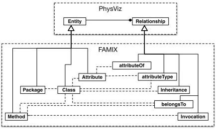
Fig. 2. Mapping code entities (from the FAMIX meta-model) to the Entities and Relationships from Figure 1.

a= 1 M

∑

FL−

D

Mv+G (2)

Where the sum is over all links to the particle and vis the current velocity of the particle. Using the standard concepts of a Newtonian point particle and Euler integration, this can easily be used to update the current position of the particle.

B. The PhysViz Asset Pipeline

We construct our physical model of a software system from two “assets”: We take a textual description of the software system itself, replete with any metrics that we wish to factor-in to our visualization, and we take a mappfactor-ing that relates the metrics to the various physical or visual properties shown in Figure 1. In games engine terms, the software system and the description of the visualisation are the designer’s input data, a representation of direction network graph is out interim build format, and the particle system is our runtime asset/object.

It is worth noting that, thanks to the separation of concerns afforded by the asset pipeline, the PhysViz framework is in principle capable of visualising anyrelational data. Although the principal purpose is to visualise software, it is not neces-sarily tied to this domain.

We adopt the definitions contained in the FAMIX meta-model [15] to discuss the entities and relationships in a software system. Thus, an entity can refer to a package, a class, a method, or a class attribute. A relationship can refer to inheritance between classes, an invocation of one method by another, the ownership of an attribute by a class, or the relationship between a class attribute and its type.

The relationship between these, and the PhysViz network model is highlighted in Figure 2. Combining this with the more detailed class diagram for PhysViz in Figure 1, it is possible to give packages, classes, methods, and attributes their own physical attributes – mass, drag, and gravity. Their various interrelationships can also be given physical properties such as length, strength, and power.

In practice, we take as input two JSON files (two assets) – one representing the software system and one representing the mappings from attributes such as metrics to physical

TABLE I SUBJECTSYSTEMS

System Classes Methods LOC

jEdit 5.2.0 1,803 9,920 155,127

Weka 3.7 3,098 23,668 429,006

properties. For our work we have constructed this file by ex-tracting the necessary information from MSE files, generated by software analysis programs such as InFusion1_.

C. Implementation

PhysViz is openly available2_{. It has been built on top of} DirectX 11. Our tool is therefore developed in C++, and is targeted towards for Windows desktops. However, the underly-ing asset build process is purely data driven, and the graphical components use standard techniques. The majority of platform specific code is in derived classes based on platform agnostic base classes, so it would be relatively straightforward to port to other platforms.

There are two possible modes in which the user can interact with PhysViz. The default mode is to use the keyboard to navigate, and to use the mouse to look around (as one would in a first-person game). Alternatively, the user can navigate with an XBox-style controller. These both being standard control methods for intuitively navigating around a 3-D environment for an increasing majority of people due to the rise of computer games.There is a further, separate component (MSE2JSON3_), which generates the input JSON files.

V. CASESTUDIES

The goal of PhysViz is to intuitively convey a large amount of information to the user without obscuring the information that might be particularly relevant to them. Here we provide a preliminary assessment of whether or not this can be achieved. We choose two openly available systems as subjects, and provide three visualisations that focus on different structural and behavioural aspects of these systems. Two of these are “physical” equivalents to established Polymetric views [9], for the sake of establishing a comparison to the state-of-the-art.

The systems considered are JEdit4, an extensible text editing program, and Weka5_{, a popular Java Machine Learning} frame-work. Their sizes (in terms of number of classes, methods and lines of code) are shown in Table I.

A. Visualisation objectives

We selected three visualisation tasks, focussing on two com-plementary aspects of a software system [21] – structure and behaviour. For the former, we introduce a PhysViz derivative of System Hotspots and System Complexity (first introduced in Lanza et al.’s Polymetric views [9]). For the behaviour perspective, we introduce the PhysViz Call Graph view. In the

1_{https://www.intooitus.com/} 2_{https://bitbucket.org/physviz/physviz}

3_{https://bitbucket.org/physviz/mse2json/overview} 4_{http://http://www.jedit.org/}

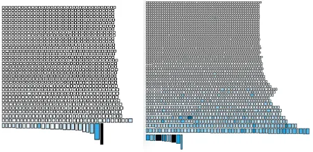
Fig. 3. Polymetric Hotspot views for JEdit (left) and Weka (right).

rest of this subsection we introduce the visualisation objectives in more detail, and present current baseline visualisations.

a) Hot spots: A hot spot visualisation should highlight classes that contain “a lot of activity”. The polymetric view for this [9] is shown in Figure 3. It represents the system as rows of boxes ordered by the number of methods (NOM). The width of each box corresponds to the number of attributes (NOA), and the height of a box corresponds to the NOM. The colour corresponds to the sum of the lines of code over all of its methods (the WLOC).

There are two inherent weakness with the visualisations shown in Figure 3. Firstly, the visualisation alone cannot be used to gauge what, for example, the actual number of methods or attributes is in any of the classes; it merely sizes them in relative terms. Secondly, for situations where a class has few methods, but where these methods are disproportionately large, this visualisation offers no means by which to compare the “hotness” of these hotspots to other hotspots with large numbers of (smaller) methods.

b) System Complexity: A system complexity visualisa-tion is intended to indicate which areas of the system are structurally particularly complex. As with the hotspot view, the complexity of individual classes (and their internal meth-ods and attributes) plays an important role. From a systems perspective however, it is important to place a class into its broader context - to incorporate the other classes in the system from which it inherits.

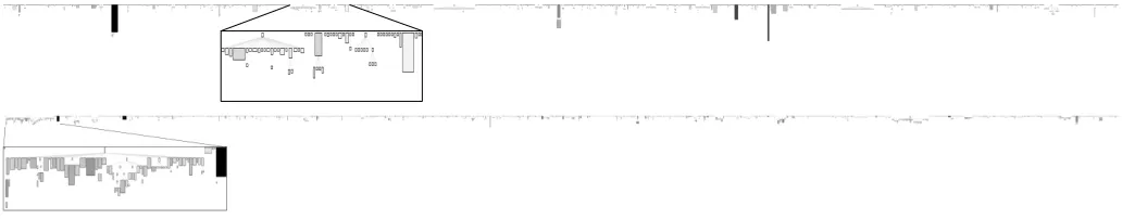
The polymetric views [9] for JEdit and Weka are shown in Figure 4. Here, classes are again given dimensions accord-ing to NOA (width), NOM (height), and WLOC (colour). However, they are also arranged into their respective class hierarchies.

As can be seen from the figure, for any reasonably large system a high degree of zooming is required to home-in on areas of interest. As with the hotspots view, the eye is drawn to big, dark classes that stand out from the rest. However, very large classes can distract from large inheritance hierarchies with lots of smaller classes (even though these can be just as intricate and complex from an engineering standpoint).

c) Call Graph View: Call graphs provide an overview of which methods in a system invoke each other at run-time. This can provide insights into what the potential modules are

TABLE II PHYSVIZCONFIGURATIONS

Hot Spot

Class M =1.0, D =5.0, G =−1.0

Method M =1.0, D =1.0, G =0.1∗LOC Attribute M =1.0, D =1.0, G =2.0

belongsTo S =1.0, P =1.0, L =10.0

System Complexity

Class M =N OM, D =N OM, G =−1.0

Method M =0.05∗LOC, D =1.0, G =−0.05∗LOC Attribute M = 1.0, D = 1.0, G = 1.0

belongsTo S =5.0, P =1.0, L =5.0

attributeOf S =1.0, P =1.0, L =5.0

inheritsFrom S =4.0, P =1.0, L =30.0

Call Graph Analysis

Class M =N OA, D =N OA, G =−1.0∗N OACCM

Method M =0.1∗LOC, D =0.2∗LOC, G =0.1∗LOC belongsTo S =2.0, P =1.0, L =2.0

calls S =1.0, P =1.0, L =50.0

within the system, or which classes are functionally related to each other [22].

As with the above visualisation tasks, there are several ex-isting means by which to visualise call graphs [23]. Traditional visualisation approaches have adopted traditional graph layout algorithms (e.g. force-directed layouts), or more recently, Holten’s Hierarchical Edge Bundling view [24].

In these traditional visualisations, the layout of the final graph is entirely determined by its topology and the choice of layout algorithm. The metrics of the nodes have no effect on the layout, even though they could clearly play a useful role (e.g. for grouping together classes according to complexity). Also, the process of rendering can be slow (Teleaet al. [23] mention that the baseline in their paper took 2 minutes to render a relatively small call graph).

B. PhysViz Configurations

The process of selecting the parameters requires a degree of judgement and adjustment to ensure that the resulting visualisation is navigable and readable. We adopt an iterative approach. The first iteration assigns the desired metrics and scales to the key parameters. Since extreme values (e.g. giving an object a mass of zero) could result in pathological behaviour (the entire software system shooting off into the distance), the second iteration focussed on ensuring the use of scales, and maximum / minimum values, to ensure that even with extreme metrics, the system does not shoot-off, and is easy to navigate. This process of parameter selection is further discussed in Section V-D.

The configurations are summarised in Table II. Any entities or relationships that are absent are also absent in the model. For space reasons we only cover the key parameters here; elements such as colour and size are left out. The full JSON configuration files for each configuration are available in the supplementary material for this paper.

Fig. 4. Polymetric System Complexity views for JEdit (top) and Weka (bottom). In both cases, parts have been magnified to highlight the structural aspects.

smaller physical objects – their methods and attributes. Meth-ods and attributes are given an intrinsic gravity (computed relative to their LOC) that draws them upwards. The gravity and mass of attributes is fixed. The end effect is that classes with large methods and lots of attributes will be dragged upwards more quickly than smaller classes with fewer, small methods. Alongside the physical attributes, we also tie the visual width and height of the methods to their LOC, so that larger methods appear visually larger. Similarly, the size of a class is relative to its NOM.

b) System Complexity: We “anchor” any classes that do not have any ancestors on a plane alongxandz. Classes are linked to each other by inheritance links, and each class is again attached to its methods and attributes. This time, each method and attribute is given a negative gravity and mass that is proportional to its LOC (more complex methods pull downwards). We also give the inheritance relationship some “springiness”, so that the relationship is stretched if it is pulled by a great force. The effect is that class hierarchies are all hanging alongside each other (as in the polymetric view). However, in our hierarchies, the complex classes should be dragged down further by the weight of their methods and attributes, making them stand out more.

c) Call Graph View: For the methods, we adopt the same gravity, mass, and drag settings as we did for the Hotspot view. Methods gravitate upwards depending on their size, and drag classes along with them. Conversely, trivial methods and their classes are not lifted up. In this visualisation, methods are connected to each other by call edges. In contrast to the edges that link methods to classes (which are short and firm), the call edges are relatively long and springy. The end-effect is that the scene should arrange itself into “clusters” of activity, where relatively isolated groups of methods that carry out a well-defined function stand out from the rest. There is also a deliberate bias, such that data-classes sink to the bottom, and function-intensive classes rise to the top.

C. Results

Given that the visualisations are inherently dynamic, it is of course difficult to provide a single figure that concisely captures what is conveyed to the user. Watching the scene unfold and monitoring the physical interactions between the classes, methods, and attributes can provide insights that cannot be conveyed by a static scene, where the elements are in fixed position.

In the results shown below, screen-shots were taken after letting the model adjust for a approximately 30 seconds6_{. The} screen shots are taken by zooming the camera into a suitable position where the vast majority of the classes are on screen. In the screen-shots, the labels have been added post-hoc. In practice, the labels appear and disappear according to the location of the POV (Point Of View). As the POV moves closer, the labels gradually appear into vision.

1) Hotspots: The hotspot screen shots are shown in Figure 5. As the simulation progresses, the classes with more methods or attributes are pulled upwards. Bigger methods pull harder, because their gravity is relative to their LOC. There are lots of small trivial classes (particularly visible at the bottom of (a), which are not pulled upwards at all. Classes are represented as “flares”, where the size and brightness is relative to the number of methods. Methods are represented as stars, where the size of the star (and its gravity and mass) are relative to the LOC.

At a glance, the screen-shots show the spread of complexity within the system. Focussing on the classes alone, just by looking at their size and brightness it is possible to determine whether the complexity is focussed on a relatively small bunch of classes (as in JEdit), or is widespread (as in Weka).

However, if we also consider the speed and direction in which the classes are being pulled, and look at the methods that are attached to them), there are further insights to be gained. In some classes, the bulk of their complexity might be contained within one or two exceptionally large methods (e.g.

BufferOptionPaneorJEditin JEdit, orEvaluation

and InstallTask in Weka. On the other hand, the com-plexity might be spread more evenly through a multitude of methods (e.g. KnowledgeFlowAppin Weka).

2) System Complexity: The System Complexity screen-shots are shown in Figure 6. As with the Polymetric views in Figure 4, the view gives a succinct impression of the extent to which inheritance has been used in the system design. In the case of JEdit, there are very few deep inheritance hierarchies. Inheritance hierarchies tend to be ‘top-heavy’; there are several large (bright pink) classes along the top, with very few large complex classes further down the hierarchy.

It is apparent that inheritance hierarchies play a greater role in WEKA. The key components of Weka [25] are the filters

6_{To begin with the entities are placed randomly, so in the first few seconds,}

Fig. 5. Hotspot screen-shots: (a) is JEdit, (b) is a close-up of CBZip2OutputStream, (c) is Weka.

(for pre-processing data), the classification algorithms, and the clustering algorithms. These are nicely reflected in Figure (b); AbstractClassifier is the root of a reasonably complex hierarchy for implementing classifiers; Filter is the root of a hierarchy for implementing various data-filters, and Clusteris the root of the hierarchy for implementing different clustering algorithms.

The physical model helps to highlight the different com-plexities of these hierarchies. Complex methods with lots of code will drag their classes down, stretching the inheritance relationship edge in the process. Looking at theSimpleNode

hierarchy in JEdit, the root class is large, has lots of methods,

and is extended by numerous very small classes. On the other hand, for theCluster hierarchy in Weka, the child classes are relatively large and complex (c.f.SimpleKMeans).

3) Call Analysis: The Call Analysis screen-shots are shown in Figure 7. The blue edges represent the calls, and the red edges represent the edges linking methods to their classes.

Fig. 6. System complexity for JEdit (a) and Weka (b).

Fig. 7. Call analysis - JEdit is shown on the left, Weka on the right.

The fact that classes are pulled-up by large methods has the effect of lowering the classes that are primarily used as data-classes to the lower area. Call edges are also coloured in a gradient from dark blue to white to indicate the direction of the edge (white represents the destination of the edge). Any method that has lots of dark-blue edges is producing lots of calls, whereas any method with lots of white edges is receiving lots of calls.

This in turn presents a useful starting point for exploring the system, both in terms of what the key data-concepts are, and for determining data-classes that potentially need to be re-engineered. Classes in the lower area of the call graph (few notably complex methods and lots of accessor methods), with

lots of white edges (lots of incoming calls and few outgoing ones) represent probable data containers.

WEKA presents a nice example of this. Figure 8 shows the lower area of the bulk of the call graph. Here, one class stands out – ResultsMatrix has mostly incoming calls (it makes several internal calls, but not to other classes in the system). As confirmed by the Weka API - ResultMatrix isa container for the datasets and classifier setups and their statistics.

D. Discussion

Fig. 8. Data-classes at the bottom of the WEKA call graph

are achieved by the same underlying physical model, and by just changing the parameters (via the mapping files). Thanks to the asset pipeline, it becomes very easy for the developer to experiment with different configurations, to gain different insights into a software system.

One striking feature about this Particle Systems-driven approach is that there is continuous feedback to the user. Whereas traditional software visualisations can take several minutes to compute and render a fixed layout, the user can watch and interact with the visualisation as it unfolds.

From a navigation perspective, some of the visualisations can become challenging to navigate when the POV is in amongst the bulk of the entities and relationships. For example, with respect to the call graph visualisation, the most valuable insights (the general structural amalgamations) are observed from afar. If the user tries to navigate to the centre of the calls, it can rapidly become disorientating. This can to an extent be mitigated by pausing the scene (to make it easier to gain a point of reference). Our ongoing work is investigating approaches by which to make it easier to navigate through denser regions.

VI. RELATEDWORK

Within the field of software visualisation, there has been a substantial amount of work on trying to address the dimen-sionality problem. Several authors have proposed the use of more sophisticated 3D visualisations, and even games engines to visualise software. Metrics-based visualisation is also well established. In this section we consider some of these key approaches, and contrast them to PhysViz.

a) 3D metrics-based software visualisation: 3D software visualisation has long been advocated, because it presents an intuitive means by which to project and navigate through a large amount of information [10]. Several techniques such as those proposed by Lewerentz et al., [26], [27] or Graham et al. [5], and Wettel and Lanza [3] enable a software system to be projected onto a 3D scene. Their essential framework

is similar to ours; software is parsed, and the metrics are used for projection in a 3D space. However, there are several important differences. For one, the final visualisation is a static scene, whereas ours is dynamic. They rely on a fixed algorithm by which to calculate distances between objects (assisted by techniques such as Principal Analysis), whereas ours is underpinned by a physics engine. Finally, their approach does not use elements such as the Artefact Pipeline, which afford a significant degree of customisability.

b) Games engines: Balogh and Beszdes introduced CodeMetropolis [4] - a code visualisation in the popular MineCraft games environment. The analogy used in their visualisation is essentially similar to that of CodeCity - files are “sky-scrapers” - albeit ones that are built out of blocks. However, given that the program is in MineCraft, it is easier to use the game navigation infrastructure to interact with and explore the environment. Although the use of games engines is similar to PhysViz, CodeMetropolis does not link metrics to physical properties such as gravity, and the layout is correspondingly not dynamic (it is restricted to Wettel’s city-block analogy [3]).

c) Graph clustering with software metrics: PhysViz is related to a line of work that has investigated the use of generic clustering algorithms to group software metrics [28]. The underlying rationale for this line of work is not necessarily visualisation or exploration, but to investigate questions with respect to the similarity of code elements, to inform tasks such as software restructuring. However, any clusterings also pro-duce “distances” between software elements, which can also form the basis for software visualisation. One problem with such clustering algorithms is that the results can sometimes be difficult to explain. For example, two classes might be clustered together because they happen to have variables with similar names, but this might not be visible or apparent to the person visualising the clusters. This problem is attenuated with PhysViz, because the rules by which elements are attracted to or repelled from each other are provided in (we argue) more intuitive, physical terms.

VII. CONCLUSIONS ANDFUTUREWORK

We have presented PhysViz, a system that makes extensive use of Games technology to produce dynamic, explorable visualisations of software systems. Thanks to the use of par-ticle models, software elements can be given various physical attributes such as mass and gravity, and the user is able to explore their interactions as they take place.

The added insights are largely thanks to the addition of physical dimensions to software entities. Nearly 20 years ago, in their work on cognition and software visualisation, Petreet al.[13] argued against the development of approaches such as PhysViz:

Dimensional restraint will be best discovered by [. . . ] devising new coding strategies for informa-tional challenges. This means breaking out of the shallow (but entertaining) concerns of building sexy virtual reality systems and thinking a lot harder about what to do with the two dimensional display devices that are already in front of our eyes.

Though eminently sensible at the time, we posit that today their stance might be different. Technology has advanced to a point where typical desktop PCs are equipped with powerful graphics devices, and games engines are widely available (not to speak of the games consoles that are as ubiquitous). It surely makes sense to make use of the advanced physical and graphical models that are afforded by such devices. Indeed, what were then high-end “sexy virtual reality systems” are becoming increasingly main-stream, with the release of a number of consumer product level head-mounted display devices: Oculus Rift, Morpheus, SteamVR. Along with people generally having a higher-level of experience of navigating through 3-D generated computer environments via activities such as computer gaming.

Our current work is focussing on ways to refine the tool. We are especially focussing on ways by which to improve navigation through crowded scenes. One approach that offers potential is to make the scene interactive, by creating a special particle representing the Point of View, that repels other particles, to give the effect of pushing them aside as the viewer moves through the system.

For our future work, we will carry out a user-study to fully explore the role of physical models, and the PhysViz exploration environment, in users’ understanding of software systems. Our second priority is to explore the various exciting opportunities for software exploration that Games Technology offers. It is for example reasonably straightforward to enable the use of immersive VR devices such as the Oculus Rift7, or more sophisticated interaction devices such as the Microsoft Kinect8 and the LEAP motion 9 . As well as apply the split-screen and multi-controller concepts of local multi-player to allow collaborative exploration of a visualisation.

REFERENCES

[1] Brooks, Frederik P., and No Silver Bullet. ”Essence and accidents of software engineering.” IEEE computer 20, no. 4 (1987): 10-19. [2] Caserta, Pierre, and Olivier Zendra. ”Visualization of the static aspects

of software: a survey.” IEEE transactions on visualization and computer graphics 17.7 (2011): 913-933.

[3] Wettel, Richard, and Michele Lanza. ”Visualizing software systems as cities.” Visualizing Software for Understanding and Analysis, 2007. VISSOFT 2007. 4th IEEE International Workshop on. IEEE, 2007.

7_{https://www.oculus.com/}

8_{https://www.microsoft.com/en-us/kinectforwindows/} 9_{https://www.leapmotion.com/}

[4] Balogh, Gergo, and Arpd Beszdes. ”CodeMetropolis-code visualisation in MineCraft.” Source Code Analysis and Manipulation (SCAM), 2013 IEEE 13th International Working Conference on. IEEE, 2013.

[5] Graham, Hamish, Hong Yul Yang, and Rebecca Berrigan. ”A solar system metaphor for 3D visualisation of object oriented software met-rics.” Proceedings of the 2004 Australasian symposium on Information Visualisation-Volume 35. Australian Computer Society, Inc., 2004. [6] Demeyer, Serge, Stphane Ducasse, and Oscar Nierstrasz. Object-oriented

reengineering patterns. Elsevier, 2002.

[7] Von Mayrhauser, Anneliese, and A. Marie Vans. ”Program comprehension during software maintenance and evolution.” Computer 28.8 (1995): 44-55.

[8] Kitchenham, Barbara, and Shari Lawrence Pfleeger. ”Software quality: The elusive target.” IEEE software 13.1 (1996): 12-21.

[9] Lanza, Michele, and Stphane Ducasse. ”Polymetric views-a lightweight visual approach to reverse engineering.” Software Engineering, IEEE Transactions on 29.9 (2003): 782-795.

[10] Teyseyre, Alfredo Ral, and Marcelo R. Campo. ”An overview of 3D software visualization.” Visualization and Computer Graphics, IEEE Transactions on 15.1 (2009): 87-105.

[11] Basili, Victor R. ”Software modeling and measurement: the

Goal/Question/Metric paradigm.” (1992).

[12] Lanza, Michele, and Radu Marinescu. Object-oriented metrics in prac-tice: using software metrics to characterize, evaluate, and improve the design of object-oriented systems. Springer Science & Business Media, 2007.

[13] Petre, Marian, A. F. Blackwell, and T. R. G. Green. ”Cognitive questions in software visualization.” Software visualization: Programming as a multimedia experience (1998): 453-480.

[14] Stasko, John, ed. Software visualization: Programming as a multimedia experience. MIT press, 1998.

[15] Ducasse, Stphane, et al. ”MSE and FAMIX 3.0: an interexchange format and source code model family.” (2011).

[16] UNITY 3D, http://unity3d.com/

[17] Unreal Engine, https://www.unrealengine.com/

[18] Tarr, P., Ossher, H., Harrison, W., & Sutton Jr, S. M. (1999, May). N degrees of separation: multi-dimensional separation of concerns. In Proceedings of the 21st international conference on Software engineering (pp. 107-119). ACM.

[19] James, Glyn. Modern engineering mathematics. Pearson Education, 2007.

[20] Eades, Peter. ”A heuristics for graph drawing.” Congressus numerantium 42 (1984): 146-160.

[21] Pacione, M. J., Roper, M., & Wood, M. A novel software visualisation model to support software comprehension. Proceedings. 11th Working Conference on Reverse Engineering (pp. 70-79). 2004.

[22] Walkinshaw, N., Roper, M., & Wood, M. Feature location and extraction using landmarks and barriers. IEEE International Conference on Software Maintenance (pp. 54-63), (ICSM), 2007.

[23] Telea, A., Hoogendorp, H., Ersoy, O., & Reniers, D. . Extraction and visualization of call dependencies for large C/C++ code bases: A comparative study. In 5th IEEE International Workshop on Visualizing Software for Understanding and Analysis (VISSOFT). (pp. 81-88). 2009. [24] Holten, D. (2006). Hierarchical edge bundles: Visualization of adjacency relations in hierarchical data. Visualization and Computer Graphics, IEEE Transactions on, 12(5), 741-748.

[25] Hall, M., Frank, E., Holmes, G., Pfahringer, B., Reutemann, P., & Witten, I. H. (2009). The WEKA data mining software: an update. ACM SIGKDD explorations newsletter, 11(1), 10-18.

[26] Lewerentz, Claus, and Frank Simon. ”Metrics-based 3D visualization of large object-oriented programs.” Visualizing Software for Understanding and Analysis, 2002. Proceedings. First International Workshop on. IEEE, 2002.

[27] Balzer, Michael, et al. ”Software landscapes: Visualizing the structure of large software systems.” (2004).

[28] Chiricota, Yves, Fabien Jourdan, and Guy Melanon. ”Software com-ponents capture using graph clustering.” Program Comprehension, 2003. 11th IEEE International Workshop on. IEEE, 2003.

[29] Nystrom, Robert. ”Game programming patterns.” Genever Benning, 2014.