Gradient based particle filter algorithm for an ARX model with nonlinear communication output

(1)

Gradient based particle filter algorithm for an ARX

model with nonlinear communication output

Jing Chen, Yanjun Liu, Feng Ding, Quanmin Zhu

Abstract—A stochastic gradient based particle filter algorithm is developed for an ARX model with nonlinear communication output in this paper. This non-standard ARX model consists of two submodels, one is a linear ARX model and the other is a nonlinear output model. The process outputs (outputs of the linear submodel) transmitted over a communication channel are unmeasureable, while the communication outputs (outputs of the nonlinear submodel) are available, and both of the two-type outputs are contaminated by white noises. Based on the rich input data and the available communication output data, a stochastic gradient based particle filter algorithm is proposed to estimate the unknown process outputs and parameters of the ARX model. Furthermore, a direct weight optimization method and the Epanechnikov kernel method are extended to modify the particle filter when the measurement noise is a Gaussian noise with unknown variance and the measurement noise distribution is unknown. The simulation results demonstrate that the stochastic gradient based particle filter algorithm is effective.

Index Terms—Parameter estimation, stochastic gradient, par-ticle filter, auxiliary model, ARX model.

I. INTRODUCTION

The non-standard ARX model which is a standard ARX model mixed with a nonlinear communication output model, can be seen as a networked control system [1], [2]. Its basic structure is shown in Fig. 1, which consists of two submodels, one is an ARX model given by

A(d)x(t) =B(d)u(t) +v(t),

and the other is a nonlinear communication output model written as

y(t) =f(x(t)) +e(t),

where u(t) is the input, x(t) is the output of the ARX model and

influenced by the process noisev(t),y(t)is the output of the

com-munication network and influenced by the measurement noisee(t),

u(t)andy(t)are measureable, whilex(t)is unmeasureable,f(·)is a known continuous nonlinear function,v(t)ande(t)are independent and identically distributed Gaussian noises with variances ς2 and σ2

, respectively, andA(d)and B(d) are polynomials which can be

expressed as

A(d) := 1 +a1d−1+· · ·+and−n,

B(d) :=b1d−1+b2d−2+· · ·+bmd−m,

where d−1x(t) = x(t−1). Different from the traditional

non-J. Chen is with School of Science, Jiangnan University, Wuxi 214122, PR China ([email protected])

Y.J. Liu and F. Ding are with Key Laboratory of Advanced Process Control for Light Industry (Ministry of Education), Jiangnan University, Wuxi 214122, PR China (yanjunliu [email protected], [email protected])

Q.M. Zhu is with Department of Engineering Design and Mathematics, Uni-versity of the West of England, Bristol BS16 1QY, UK ([email protected]) This work is supported by the National Natural Science Foundation of China (No. 61403165) and the Natural Science Foundation for Colleges and Universities in Jiangsu Province (No. 16KJB120006)

- B(d)

A(d) -+lp p p p p p p p p p p p- f(·) p p p p p p p p p p p p-+l

-?

1

A(d)

? ?

u(t) x(t) y(t)

v(t)

[image:1.612.315.547.171.268.2]

e(t)

Fig. 1. The ARX model with nonlinear communication output

linear models, such as the Hammerstein model, the Wiener model or the Hammerstein-Wiener-Hammerstein model, the non-standard ARX model has two submodels and has two kinds noises, thus the identification for this model is more difficult. Recently, this type of model is usually considered in process control and estimation literature [3], [4]. Under such a scenario, the process outputs are often sampled by some sensors and are typically sent to a laboratory for analysis. Due to the complexities of communication network and laboratory analysis process, these outputs as the laboratory analysis outcomes can have nonlinear properties as well as their own errors from the laboratory analysis. The focus of this paper is to develop an on-line identification algorithm for the non-standard ARX model whose measurement noise has different properties.

The ARX model identification has been extensively studied in theory [5], [6]. Many identification methods, such as the recursive least squares (RLS) algorithms [7], the hierarchical algorithms [8], the stochastic gradient (SG) algorithms [9] and the iterative algorithms [10], have been proposed for ARX models. The hierarchical algo-rithms decompose the complex model into several submodels with small dimensions and then coordinate the associate terms between submodels [11]. The iterative algorithms are off-line algorithms which have heavy computational efforts and cannot be used to estimate the parameters recursively by new data, while the RLS and SG algorithms can be used as on-line algorithms and can update the parameters based on new data. Furthermore, these on-line algorithms have less computational efforts, thus widely used in engineering application.

The on-line algorithms often have the assumption that all the system data are available. However, in engineering practice, some data of the systems may be missing or unmeasureable. The auxiliary model is an important tool which is usually applied for systems with missing data [12]. Its basic idea is to replace the missing data with the outputs of an auxiliary model. For example, Wang and Ding studied an auxiliary model based RLS algorithm for multivariable systems [13]. Jin et al investigated an auxiliary model based identification algorithm for multivariable OE-like systems with missing outputs [12]. Such methods only use an auxiliary model to predict the missing outputs, while the measureable outputs are not applied to improve the predicted outputs, which makes the auxiliary model have slow convergence rates.

(2)

analysis process also bring some identification constraints, such as the packet dropouts, the communication time-delays, the nonlinear signals and the unmeasureable sampled outputs [17]–[19]. There exist many identification methods for systems with such constraints. For example, Guo et al proposed an identification algorithm for FIR systems, in which the outputs are constrained by both the binary-valued quantization and the communication unreliability [20]. Xiong et al investigated an EM algorithm for nonlinear systems with unmeasureable outputs, in which those unmeasureable outputs were estimated by an auxiliary model [21]. Xie et al developed an EM algorithm for multi-rate systems with random time-delays, where the output model is linear and the process model is not influenced by process noise, by using an auxiliary model and an off-line algorithm, the missing outputs and the parameters were estimated simultaneously [22].

The Kalman filter and the particle filter are two effective tools which are often applied for state-space systems [23]–[25]. In [26], a Kalman filter based off-line algorithm is derived for state-space systems, and in order to enhance the computational efficiency, a model decomposition based off-line algorithm is also provided. In [3], an EM based particle filter algorithm is proposed for nonlinear parameter varying state-space systems, where the proposed EM algorithm is an off-line algorithm. Unlike the auxiliary model, the Kalman filter and the particle filter apply the measureable data to improve the priori estimates, which makes them be more accurate. However, these two filters are often used for state-space systems.

This paper takes the above described literature into study and develops an SG based particle filter algorithm for an ARX model with nonlinear communication output. The considered system in this paper is a non-state-space system with different kinds of measurement noises, and the proposed algorithm is an on-line algorithm. A particle filter is derived to estimate the process outputs by the communication outputs. Then based on the estimated process output data and the rich input data, the unknown parameters can be estimated by an SG algorithm. The problem discussed in this paper is more complicated and challenging than those in [3], [4], [22] and the main contributions are listed below.

1) Study an on-line identification method for a non-standard ARX model which consists of two submodels, one is the ARX model to reflect process dynamics, and the other is an equation reflecting nonlinear output.

2) Propose a particle filter instead of an auxiliary model for nonlinear non-state-space systems, which can estimate the unknown variables and can increase the estimation accuracy. 3) Apply the direct weight optimization method and the

Epanech-nikov kernel method to modify the particle filter for the situations that the measurement noise with unknown variance and unknown distribution.

Briefly, the rest of this paper is organized as follows. Section II presents an SG based particle filter algorithm. Section III develops two modified particle filters. In Section IV, three illustrative examples are provided. Section V concludes this paper and gives future directions.

II. THESGBASED PARTICLE FILTER ALGORITHM

For the model depicted in Fig. 1, define the information vector

φ(t)and the parameter vectorθas

φ(t) := [−x(t−1),· · ·,−x(t−n), u(t−1),· · ·, u(t−m)]T_∈_Rn+m

,

θ:= [a1,· · ·, an, b1,· · ·, bm]T∈Rn+m,

then the non-standard ARX model can be rewritten as follows,

x(t) =φT

(t)θ+v(t), (1)

y(t) =f(x(t)) +e(t). (2)

In Equation (1), the information vector contains unknown process outputsx(i), i= 1,2,· · ·, thus the classical SG algorithm cannot be

applied to (1) directly. The auxiliary model based algorithms are often used to identify systems with unmeasureable variables [27], [28]. For example, the corresponding auxiliary model based SG (AM-SG) algorithm for the system model in (1) and (2) is below,

ˆ

θ(t) = ˆθ(t−1) +φˆ(t)

ν(t)ϵ(t), (3)

ˆ

φ(t−i) = [−x(tˆ −i−1),· · ·,−x(tˆ −i−n), u(t−i−1),· · ·, u(t−i−m)]T

, (4)

ˆ

x(t−i) = ˆφT

(t−i)ˆθ(t−i−1), (5)

ϵ(t) =x(t)−φˆT

(t)ˆθ(t−1), (6)

ν(t) =ν(t−1) +∥φˆ(t)∥2, ν(0) = 1, (7) in whichθˆ(t−i−1)is the estimate ofθatt−i−1. However, here the SG-AM algorithm cannot be applied to deal with this non-standard model.

Remark 1: Unlike the models in [27], [28], all the process outputs in this non-standard ARX model are unknown, and if we usex(t) =ˆ

ˆ

φT_(t)ˆ_θ_(t₋₁₎_{to replace}_x(t)_{, then}_ϵ(t)_{in Equation (6) becomes zero,}

thus the SG-AM algorithm proposed in Equations (3)-(7) is invalid for this non-standard ARX model.

The key characteristic of our treatment is to develop a particle filter based on-line algorithm for this non-standard ARX model.

A. The particle filter

The particle filter is a tool for nonlinear state-space systems with unmeasureable states. In what follows we will extend this tool to nonlinear non-state-space systems.

The basic idea of the particle filter is to use a series of particles with associated weights to approximate the posterior density function. Based on the particle filter method in [3], [29], the posterior density functionp(x(t−i)|y(t−i),· · ·, y(1), x(t−i−1),· · ·, x(1), u(t−

i−1),· · ·, u(1))can be approximately as

p(x(t−i)|y(t−i),· · ·, y(1), x(t−i−1),· · ·, x(1),

u(t−i−1),· · ·, u(1),θˆ(t−i−1))

≈

N ∑

j=1

ωjδ(x(t−i)−xˆj(t−i)), (8)

whereωj is the normalized weight associated with thejthparticle

andδ(·)denotes the Dirac delta function. Once the particles and their weights have been obtained, we can compute any desired statistical measure of the posterior density function. For example, the mean of the posterior density function can be computed as

ˆ

x(t−i) =

N ∑

j=1

¯

ωjxˆj(t−i), (9)

in whichω¯j= ωj N ∑ j=1

ωj

is the weight associated with thejthparticle

and

N ∑

j=1

¯

ωj = 1, xˆj(t−i) is the jth particle drawn from the

posterior density functionp(x(t−i)|y(t−i),· · ·, y(1), x(t−i−

1),· · ·, x(1), u(t−i−1),· · ·, u(1),θ). However, it is difficult to

draw particles from this posterior density function directly. In order to get the new particles, an importance densityq(·)is given by,

q(x(t−i)|y(t−i),· · ·, y(1), x(t−i−1),· · ·, x(1),

u(t−i−1),· · ·, u(1),ˆθ(t−i−1))

=p(x(t−i)|x(t−i−1),· · ·, x(1),

u(t−i−1),· · ·, u(1),ˆθ(t−i−1)). (10)

From Equations (1) and (10), one gets

(3)

u(t−i−1),· · ·, u(1),θˆ(t−i−1))

=√1 2πςexp

[

−(x(t−i)−φT(t−i)ˆθ(t−i−1))2

2ς2

]

. (11)

Remark 2: If the varianceς is unknown, then the density function in Equation (11) would not be computed, and the particles could not be updated. In this scenario, the auxiliary model can be applied to draw the particles, e.g.,

ˆ

xj(t−i) = ˆφTj(t−i)ˆθ(t−i−1),

ˆ

φj(t−i) = [−ˆxj(t−i−1),· · ·,−xˆj(t−i−n),

u(t−i−1),· · ·, u(t−i−m)]T

,

whereθˆ(t−i−1)is the estimate ofθat timet−i−1.

From Equation (11), we can get the new particles. The next is to update the weight of each new particle. Based on [3], the weight ωj(t)can be updated as follow,

ωj(t) =p(y(t)|xˆj(t))ωj(t−1). (12)

According to Equation (2), the density functionp(y(t)|xˆj(t))can

be computed by

p(y(t)|xˆj(t)) =

1

√

2πσexp

[

−(y(t)−f(ˆxj(t)))2

2σ2

]

. (17)

Substituting (17) into (16) gets

ωj(t) =

1

√

2πσexp

[

−(y(t)−f(ˆxj(t)))2

2σ2

]

ωj(t−1). (18)

Normalizingωj(t)yields

¯ ωj(t) =

ωj(t) N ∑ j=1

ωj(t)

. (19)

Then we have

ˆ

x(t−i) =

N ∑

j=1

¯

ωj(t−i)ˆxj(t−i). (20)

When apply the particle filter to estimate the unknown variables, the degeneracy phenomenon is an inevitable problem [30]. After a few iterations, the weights of some particles become small, which means that heavy computational efforts are utilized to update those particles whose contributions are negligible. In order to avoid this phenomenon, a sample sizeNef f is defined as,

Nef f:= [_N

∑

j=1

¯ ωj(t)2

]−1

. (21)

Given a threshold Nhold in prior, Nef f < Nhold means severe

degeneracy. Thus we should use resampling, and then the weight of each particle is assigned asω¯j=_N1.

The particle filter proceeds by performing the following steps.

1) Initialization: At time t, collect the input-output

da-ta {u(1), y(1),· · ·, u(t), y(t)}. Draw N initial particles

{xˆj(0)}Nj=1fromp(x(0)|θˆ(t−1))and set{ωj(0)}Nj=1=N1,

ˆ

θ(t−1)is the estimate ofθat timet−1. 2) Let the process noise variance beς2

and the measurement noise variance beσ2

, and assign a positive numberNhold.

3) Leti=t−1.

4) Compute {xˆj(t−i)}Nj=1from Equation (11).

5) Compute ωj(t−i)by Equation (18).

6) Normalizeω¯j(t−i) from Equation (19).

7) Compute the missing outputx(tˆ −i)by Equation (20).

8) Compute Nef f by Equation (21) and compare Nef f with

Nhold, if Nef f < Nhold, reset the weight of each particle

withω¯j(t−i) = _N1 and go to next step; otherwise, go to next

step.

9) Let i=i−1, ifi>0go to step 4; otherwise terminate the procedure.

B. The identification algorithm

In order to estimatex(t), two methods are discussed here. One is to keep the estimates of the unknown process outputs at timet−i−2 unchanged, while we only useˆθ(t−i−1)to estimatex(t−i).

DrawNparticles from the following importance density function,

q(x(t−i)|y(t−i),· · ·, y(1),x(tˆ −i−1),· · ·,x(1),ˆ

u(t−i−1),· · ·, u(1),θˆ(t−i−1)), (22)

in which

ˆ

x(t−i−1) = [x(t−i−1)]|ˆ

θ(t−i−2),

.. . ˆ

x(1) = [x(1)]|ˆ

θ(0),

where[x(t−i−j)]_θˆ

(t−i−j−1), j= 1,· · ·, i−1means the estimate

ofx(t−i−j)by usingθˆ(t−i−j−1). Based on Equation (20), we can get the estimatex(tˆ −i). Then with the estimates {x(tˆ −

i),x(tˆ −i−1),· · ·,x(1)ˆ }andθˆ(t−i−1), one can get the parameter

estimateθˆ(t−i).

From (22), we can see that only one process output datax(t−i) is required to be estimated at each sampling timet−i−1.

Unlike the first method, in order to get the parameter estimates att−i, the second method is to estimate all the unknown process outputs up to and including timet−iby using the parameter estimate ˆ

θ(t−i−1).

DrawN particles from

q(x(t−i)|y(t−i),· · ·, y(1),x(tˆ −i−1),· · ·,x(1),ˆ

u(t−i−1),· · ·, u(1),θˆ(t−i−1)), (23)

in which

ˆ

x(t−i−1) = [x(t−i−1)]|ˆ

θ(t−i−1),

.. . ˆ

x(1) = [x(1)]|ˆ

θ(t−i−1).

From Equation (20), we can obtain the estimates x(tˆ −i). Then

according to the estimates{x(tˆ −i),x(tˆ −i−1),· · ·,x(1)ˆ } and ˆ

θ(t−i−1), we can get the updated parameter vectorθˆ(t−i). The density function in (23) declares that one should estimatet−i process outputs at each sampling timet−i−1.

Remark 3: The estimates of the process output data by using the second method are more accurate than those by using the first method. However, compared with the first method, the second method has heavier computational efforts.

In order to estimate the unmeasureable data more accurately, we use the second method in this paper. Then the SG based particle filter (SG-PF) algorithm is given by,

ˆ

θ(t) = ˆθ(t−1) +φˆ(t)

r(t)[ˆx(t)−φˆ

T

(t)ˆθ(t−1)], (24)

ˆ

φ(t) = [−x(tˆ −1),· · ·,−x(tˆ −n), u(t−1),· · ·,

u(t−m)]T, (25)

ˆ

x(t−i) =

N ∑

j=1

¯

ωj(t−i)ˆxj(t−i), (26)

r(t) =r(t−1) +∥φˆ(t)∥2, r(0) = 1. (27) The SG-PF algorithm proceeds by performing the following steps. 1) Let u(t) = 0,x(t) = 0, y(t) = 0ˆ , t 6 0, and give a small

positive numberε.

2) Lett= 1, ˆθ(0) = [1/p0,· · ·,1/p0]T∈Rn+m, wherep0 =

106.

(4)

ωj(t) =

p( ˆXj(t), Y(t),θˆ(t−1))

q( ˆXj(t)|Y(t),θˆ(t−1))

= p(ˆxj(t), y(t),

ˆ

Xj(t−1), Y(t−1),ˆθ(t−1))

q(ˆxj(t)|Xˆj(t−1), Y(t),ˆθ(t−1))q( ˆXj(t−1)|Y(t),θˆ(t−1))

= p(y(t)|xˆj(t),

ˆ

Xj(t−1), Y(t−1),θˆ(t−1))p(ˆxj(t)|Xˆj(t−1), Y(t−1),θˆ(t−1))p( ˆXj(t−1), Y(t−1),ˆθ(t−1))

q(ˆxj(t)|Xˆj(t−1), Y(t),θˆ(t−1))q( ˆXj(t−1)|Y(t−1),θˆ(t−1))

= p(y(t)|xˆj(t),

ˆ

θ(t−1))p(xj(t)|xˆj(t−1),· · · ,ˆxj(1), u(t−1),· · ·, u(1),θˆ(t−1))

q(xj(t)|y(t),· · · , y(1),xˆj(t−1),· · · ,xˆj(1), u(1), u(2),· · · , u(t−1),θˆ(t−1))

ωj(t−1)

=p(y(t)|xˆj(t))ωj(t−1). (16)

4) Update ω¯j(t−i) and xˆj(t−i), j = 1,· · ·, N by using the

particle filter.

5) Compute ˆx(t−i), i=t−1, t−2,· · ·,0by Equation (26). 6) Formφˆ(t)by Equation (25).

7) Compute r(t)by Equation (27).

8) Estimateθˆ(t)by Equation (24).

9) Letτ =∥ˆθ(t)−ˆθ(t−1)∥/∥θˆ(t)∥, ifτ 6ε, then obtain the estimated parameter vectorˆθ(t); otherwise, lett=t+ 1and go back to step 3.

Remark 4: From the SG-PF algorithm in (24)-(27), we can see that the unknown process output is estimated by Equation (26), obviously, ˆ

x(t)−φˆT

(t)ˆθ(t−1)̸= 0. Thus the SG-PF algorithm can be utilized to estimate the unknown parameters.

III. TWO MODIFIED PARTICLE FILTERS

In the above section, we assume that the measurement noise is a Gaussian noise with known variance. However, in engineering practice, the variance of the Gaussian noise is often unknown. More-over, the distribution of the measurement noise may be unknown. In this section, we consider the cases that the measurement noise is a Gaussian noise with unknown variance and the measurement noise distribution is unknown, and develop two modified particle filters to estimate the process outputs. .

A. The Gaussian measurement noise with unknown variance

Since the variance of the measurement noise is unknown, the

weight wj(t) in Equation (18) cannot be computed directly. In

order to circumvent this difficulty, we introduce a direct weight optimization method to update the weight of each particle.

DrawN particlesxˆj(t),j= 1,· · ·, N from (23) and define

p(y(t)|xˆj(t)) :=λj(t).

The next is to find the weights λj(t), j = 1,· · ·, N so that the

nonlinear functionf(x(t))can be approximated by

f(x(t))≈

N ∑

j=1

λj(t)(f(ˆxj(t)),

in which

N ∑ j=1

λj(t) = 1, λj(t) > 0. Based on the direct weight

optimization method in [31], the weights λj(t), j = 1,· · ·, N can

be obtained by minimizing the following function

[ _N ∑

j=1

λj(t)(f(ˆxj(t)) +e(t))−y(t) ]2

=

(_N ∑

j=1

λj(t)f(ˆxj(t)) + N ∑

j=1

λj(t)e(t)− N ∑

j=1

λj(t)y(t) )2

.(28)

Define

|y(t)−f(ˆxj(t))|:=γj(t).

Taking the conditional expectation on (28) yields

E

[_N ∑

j=1

λj(t)(f(ˆxj(t)) +e(t))−y(t) ]2

=

( _N ∑

j=1

λj(t)γj(t) )2

+σ2

N ∑

j=1

λ2j(t). (29)

Let

z(t) =

N ∑

j=1

λj(t)γj(t) + N ∑

j=1

|λj(t)e(t)|.

According to the direct weight optimization method proposed in [31], we can find the weights to make sure that P rob(z > γ(t)) is minimized. In this paper, we chooseγ(t)as

γ(t) = max{γj(t), j= 1,· · ·, N}+ 1.

The choice ofγ(t)can keep the number of particles unchanged and

can prevent sample impoverishment. Since the measurement noise e(t)is a Gaussian noise, the density function ofz can be expressed as

p(z) =

{ 2 √

(2π)ζ2exp (

−(z−z0)2

2ζ2 )

, z>z0,

0,

(30)

where

z0= N ∑

j=1

λj(t)γj(t), ζ=σ v u u t∑N

j=1

λ2 j(t).

MinimizingP rob(z>γ(t))is equivalent to

Max_∑N

j=1

λj(t)=1,λj(t) γ(t)−

N ∑ j=1

λj(t)γj(t)

N ∑ j=1

λ2 j(t)

.

Then the weight can be computed by

λj(t) =

γ(t)−γj(t)

N γ(t)−

N ∑

j=1

γj(t)

(5)

Substituting Equation (31) into Equation (16) gets

ωj(t) =λj(t)ωj(t−1),

and the normalized weight can be expressed as

¯ ωj(t) =

ωj(t) N ∑

k=1

ωk(t)

. (32)

Remark 5: Equations (31) and (32) imply that the weight of each particle can be obtained without the knowledge of the variance of the measurement noise.

B. The measurement noise with unknown distribution

When the distribution of the measurement noise is unknown, both the density function in Equations (17) and (30) cannot be obtained. In order to solve this problem, we use the Kernel density estimation method to update the weight of each particle.

Rewrite

|y(t)−f(ˆxj(t))|=γj(t),

γ(t) = max{γj(t), j= 1,· · ·, N}+ 1.

Sincef(·)is a continuous function, we can conclude that the smaller the γj(t)is, the more important role of thejthparticle at timetin

estimating the true outputx(t)plays. The Epanechnikov function is a significant type of kernel function and is optimal in a mean square error sense. Here, the Epanechnikov function is introduced to estimate p(y(t)|ˆxj(t))[32].

Since

γj(t)

γ(t) <1, j= 1,· · ·, N,

then the density function is given by

p(y(t)|xˆj(t)) =

3 4

[

1−(γj(t) γ(t))

2 ]

.

By normalizing the density function, one has

p(y(t)|xˆj(t)) =

γ2(t)−γ2j(t)

N γ2_(t)− N ∑ j=1

γ2 j(t)

. (33)

Substituting Equation (33) into Equation (16) gets

ωj(t) =

γ2(t)−γ2j(t)

N γ2_(t)₋ N ∑ j=1

γ2 j(t)

ωj(t−1).

Normalizingωj(t)yields

¯ ωj(t) =

ωj(t) N ∑ j=1

ωj(t)

.

Remark 6: Assume γs(t) < γl(t), 1 6 s 6 N, 16 l 6 N and

s̸=l. It follows that

γ2_(t)₋_γ2 s(t)

N γ2_(t)₋ N ∑ j=1

γ2 j(t)

> γ

2_(t)₋_γ2 l(t)

N γ2_(t)₋ N ∑ j=1

γ2 j(t)

.

It means that the sth particle plays a more important role in

estimating the estimatex(t)ˆ than thelthparticle.

Theorem 1: Assume thatp(y(t)|xˆj(t))is expressed by Equation

(33) and the distribution of the measurement noise is unknown, then the following inequality holds

N ∑

j=1

p(y(t)|ˆxj(t))(y(t)−f(ˆxj(t)))2 6 N ∑

j=1

1

N(y(t)−f(ˆxj(t)))

2

.

The detailed derivation is given in Appendix A.

Theorem 1 shows that the estimation accuracy can be improved by using the updated weights.

Remark 7: When the measurement noise is a Gaussian noise with unknown variance, the Kernel density estimation method also can be applied to update the weight of each particle. On the other hand, the direct weight optimization method cannot be utilized to update the weight of each particle when the distribution of the measurement noise is unknown.

Theorem 2: Letλdj(t) be the weight updated by Equation (31),

λkj(t) be the weight updated by Equation (33). Assume that the

measurement noise is a Gaussian noise with unknown variance, then

N ∑

j=1

λdj(t)(y(t)−f(ˆxj(t)))26 N ∑

j=1

λkj(t)(y(t)−f(ˆxj(t)))2.

The proof is given in Appendix B.

Theorem 2 means that the direct weight optimization method is the optimal method when the measurement noise is a Gaussian noise with unknown variance.

IV. EXAMPLES

Example 1:Consider an ARX model with unknown outputs,

A(d)x(t) =B(d)u(t) +v(t),

A(d) = 1 +a1d−1= 1 + 0.49d−1,

B(d) =b1d−1+b2d−2=−0.83d−1+ 0.17d−2,

and the output model is

y(t) = exp(x(t)) +e(t),

u∼N(0,1), v∼N(0, ς2), e∼N(0, σ2),

in whichx(t) is unmeasureable,y(t)is measureable, the variances of{v(t)}and{e(t)}are both0.102. In simulation, we choose100 particles.

Apply the SG-PF algorithm to estimate the parameters of the ARX model. The simulation data of the inputs, process outputs and nonlinear communication outputs are shown in Fig. 2 (samples 1-200). The parameter estimation errorsτ :=∥θˆ−θ∥/∥θ∥versus t are depicted in Fig. 3, and the parameter estimates and their errors are presented in Table I. The estimated process outputs, the true process outputs and their errors are shown in Fig. 4 (samples 800-900).

TABLE I

THESG-PFALGORITHM ESTIMATES AND ERRORS IN EXAMPLE1

t a1 b1 b2 τ(%)

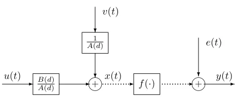
100 0.30121 -0.82158 0.03847 23.52512 200 0.37672 -0.82428 0.09128 14.10643 400 0.46706 -0.82416 0.12997 4.75154 600 0.48365 -0.82306 0.15922 1.46191 800 0.48532 -0.84526 0.17290 1.65736 1000 0.48776 -0.82236 0.16352 1.04817 True Values 0.49000 -0.83000 0.17000

Example 2: Consider the non-standard ARX model proposed in

Example 1.

A(d)x(t) =B(d)u(t) +v(t), y(t) = exp(x(t)) +e(t),

u∼N(0,1), v∼N(0, ς2).

The variance of{v(t)}is0.102, while the distribution of{e(t)}is unknown. In simulation, we also choose100particles.

Apply the Epanechnikov function to improve the weights of the

(6)

0 20 40 60 80 100 120 140 160 180 200 −2

0 2

input data

0 20 40 60 80 100 120 140 160 180 200

−2 0 2

missing data

0 20 40 60 80 100 120 140 160 180 200

0 5

output data

Simulation data

Fig. 2. The simulation data in Example 1

0 100 200 300 400 500 600 700 800 900 1000 0

0.1 0.2 0.3 0.4 0.5 0.6 0.7 0.8 0.9 1

t

[image:6.612.61.282.63.227.2]

τ

Fig. 3. The parameter estimation errorsτversustin Example 1

800 810 820 830 840 850 860 870 880 890 900 −2

−1.5 −1 −0.5 0 0.5 1 1.5 2 2.5 3

t

[image:6.612.326.545.68.313.2]

True value Prediction Estimaion errors

Fig. 4. Estimated model outputs, true outputs and estimation errors in Example 1

The estimation errors τ versus t are depicted in Fig. 5, and the

parameter estimates and their errors are presented in Table II. The estimated process outputs, the true process outputs and their errors are shown in Fig. 6 (samples 800-900).

From Examples1and2, we can get the following finds. 1) Figs. 3 and 5 show that the parameter estimation errors of

these two methods decay and finally vanish whentis increased. 2) Figs. 4 and 6 declare that the estimated outputs by the SG-PF

algorithm can track the true missing outputs.

3) Values in Tables I and II witness that the parameter estimation errors through the SG-PF algorithm with known measurement noise are smaller than those through the SG-PF algorithm with unknown measurement noise.

Example 3:Consider an experiment setup of a water tank system

in Fig. 7, where u(t) is the valve opening, and x(t) is the liquid level. There is a pressure sensor at the bottom of Tank 2 which can transmit the liquid level of Tank 2 over a communication network.

TABLE II

t a1 b1 b2 τ(%)

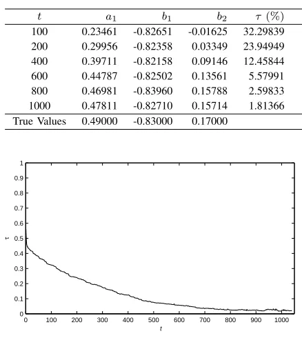
100 0.23461 -0.82651 -0.01625 32.29839 200 0.29956 -0.82358 0.03349 23.94949 400 0.39711 -0.82158 0.09146 12.45844 600 0.44787 -0.82502 0.13561 5.57991 800 0.46981 -0.83960 0.15788 2.59833 1000 0.47811 -0.82710 0.15714 1.81366 True Values 0.49000 -0.83000 0.17000

0 100 200 300 400 500 600 700 800 900 1000 0

0.1 0.2 0.3 0.4 0.5 0.6 0.7 0.8 0.9 1

t

[image:6.612.61.283.100.345.2]

τ

Fig. 5. The parameter estimation errorsτ versustin Example 2

800 810 820 830 840 850 860 870 880 890 900 −2

−1.5 −1 −0.5 0 0.5 1 1.5 2 2.5 3

t

? u(t)

p p p p p p p p p p p p p p p p p p p p p p p p p p p p p p p p p p p p p p p p p p p p p p p p p p p p p p p p p p p p p p p p p p p p p p p p p p p

Tank 1

?

Sensor

p p p p p p p p p p p p p p p p p p p p p p p p p p p p p p p p p p p p p p p p p p p p p p p p p p p p p p p p p p p p p p p p p p p p p p p p p p p

Tank 2

x(t)

p p p p p p p p pCommunication network -y(t)

Fig. 7. A water tank system

[image:6.612.330.542.353.476.2] [image:6.612.71.281.390.514.2]

(7)

following ARX model,

A(d)x(t) =B(d)u(t) +v(t),

A(d) = 1 +a1d−1+a2d−2 = 1 + 0.47d−1+ 0.18d−2,

B(d) =b1d−1+b2d−2=−0.82d−1+ 0.31d−2,

and we manually amplify the output as

y(t) =x(t) + 0.2x2(t) +e(t).

This kind of nonlinear function can be seen in [21], [33]. In simu-lation, the input{u(t)}is a filtered random binary signal sequence,

{v(t)}and {e(t)}are Gaussian white noise sequences and both of their variances are0.102_{. In simulation, we use}₅₀_particles.

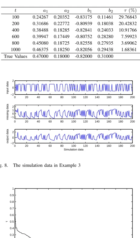
The simulation data of the inputs, process outputs and nonlinear outputs are depicted in Fig. 8 (samples 1-200). The estimation errors τversustare depicted in Fig. 9, and the parameter estimates and their estimation errors are presented in Table III. The estimated process outputs, the true process outputs and their errors are shown in Fig. 10 (samples 800-900).

TABLE III

t a1 a2 b1 b2 τ(%)

100 0.24267 0.20352 -0.83175 0.11461 29.76843 200 0.31686 0.22772 -0.80939 0.18038 20.42832 400 0.38488 0.18285 -0.82841 0.24033 10.91766 600 0.39947 0.17449 -0.80752 0.28280 7.59923 800 0.45080 0.18725 -0.82558 0.27935 3.69062 1000 0.46375 0.18250 -0.82056 0.29438 1.68361 True Values 0.47000 0.18000 -0.82000 0.31000

0 20 40 60 80 100 120 140 160 180 200

−2 0 2

input data

0 20 40 60 80 100 120 140 160 180 200

−1 0 1 2

missing data

0 20 40 60 80 100 120 140 160 180 200

−2 0 2

output data

Simulation data

Fig. 8. The simulation data in Example 3

0 100 200 300 400 500 600 700 800 900 1000 0

0.1 0.2 0.3 0.4 0.5 0.6 0.7 0.8 0.9 1

t

[image:7.612.330.543.55.180.2]

τ

Fig. 9. The parameter estimation errorsτversustin Example 3

800 810 820 830 840 850 860 870 880 890 900 −2

−1.5 −1 −0.5 0 0.5 1 1.5 2 2.5 3

t

[image:7.612.57.289.273.667.2]

From Fig. 9 and Table III, we can conclude that ast increases,

the parameter estimation errors approach zero. From Fig. 10, we find that the estimated process outputs can track the true unmeasureable outputs well.

V. CONCLUSIONS

An SG-PF algorithm is proposed for a non-standard ARX model in this paper. This model consists of two submodels, one is an ARX model and the other is a nonlinear communication output model. Since the outputs of the ARX model are unmeasureable, a particle filter is utilized to estimate these unknown outputs. Then based on the measureable input data and the estimated process output data, the unknown parameters of the ARX model can be estimated by the SG algorithm. Furthermore, two modified particle filters are developed for the non-standard ARX model with the assumptions that the measurement noise is a Gaussian noise with unknown variance and the measurement noise distribution is unknown.

The purpose of this paper is to develop an on-line identification method for systems with nonlinear communication output. There are still some interesting topics not discussed in this paper. For example, if the structure of the nonlinear function is unknown, how to adjust the weights of the particles? Another topic is how to prove the convergence properties of the SG-PF algorithm. These topics will remain as open issues in future.

APPENDIXA PROOF OFTHEOREM1

Define

|y(t)−f(ˆxj(t))|:=γj(t), j= 1,2,· · ·, N,

γ(t) := max{γj(t), j= 1,· · ·, N}+ 1.

According to Equation (33), one can get

N ∑

j=1

p(y(t)|xˆj(t))(y(t)−f(ˆxj(t)))2− N ∑

j=1

1

N(y(t)−f(ˆxj(t)))

2

=

N ∑

j=1   

 γ

2

(t)−γj2(t)

N γ2_(t)− N ∑

k=1

γ2 k(t)

− 1

N

   γj2(t)

=

N ∑

j=1

−(N−1)γ2j(t) + N ∑

k=1,k̸=j

γk2(t)

N(N γ2_(t)− N ∑ k=1

γ2 k(t))

(8)

Since the denominator of the last term of the above equation is greater than zero, one only need to consider the following equation

N ∑

j=1 

−(N−1)γj2(t) + N ∑

k=1,k̸=j

γk2(t)  γj2(t)

=

[

(1−N)γ41(t) +γ 2 1(t)

N ∑

k=2

γk2(t) ]

+· · ·



(1−N)γj4(t) +γ2j(t) N ∑

k=1,k̸=j

γk2(t) 

+· · ·

[

(1−N)γ4N(t) +γ 2 N(t)

N_∑−1 k=1

γk2(t) ]

=−

N ∑

k=2

(γ12(t)−γ 2 k(t))2−

N ∑

k=3

(γ22(t)−γ 2

k(t))2− · · ·

− N ∑

k=j+1

(γj2(t)−γ 2 k(t))

2_{− · · · −}

(γ_N−12 (t)−γN2(t)) 2₆

0.

Clearly, the following inequality holds

N ∑

j=1

p(y(t)|ˆxj(t))(y(t)−f(ˆxj(t)))2 6 N ∑

j=1

1

N(y(t)−f(ˆxj(t)))

2

.

APPENDIXB PROOF OFTHEOREM2

The weight which updated by the direct weight optimization method is expressed as

λdj(t) =

γ(t)−γj(t)

N γ(t)−

N ∑ j=1

γj(t)

, (34)

while the weight updated by the Kernel density estimation method is written by

λkj(t) =

γ2_(t)₋_γ2 j(t)

N γ2_(t)− N ∑ j=1 γ2 j(t) . (35)

Then one can get

N ∑

j=1

λdj(t)(y(t)−f(ˆxj(t)))2− N ∑

j=1

λkj(t)(y(t)−f(ˆxj(t)))2

=

N ∑

j=1

λdj(t)γ 2 j(t)−

N ∑

j=1

λkj(t)γ 2 j(t) = N ∑ k=1 γ2 k(t) [ N ∑ j=1 γ2

j(t)(γj(t)−γ(t)) ]

(

N γ(t)−

N ∑ j=1

γj(t) ) (

N γ2_(t)− N ∑ j=1 γ2 j(t) )+ N ∑ k=1

γk(t) [

N ∑ j=1

γ2

j(t)(γj(t) +γ(t))(γj(t)−γ(t)) ]

(

N γ(t)−

N ∑ j=1

γj(t) ) (

N γ2_(t)− N ∑ j=1 γ2 j(t) ) + N γ(t) [ N ∑ j=1

γj3(t)(γj(t)−γ(t)) ]

(

N γ(t)−

N ∑

j=1

γj(t) ) (

N γ2_(t)− N ∑

j=1

γ2 j(t)

). (36)

Since the denominator of Equation (36) is greater than zero, one only need to consider the numerator of Equation (36),

N ∑

k=1

γk2(t) [ _N

∑

j=1

γj2(t)(γj(t)−γ(t)) ]

+

N ∑

k=1

γk(t) [_N

∑

j=1

γ2j(t)(γj(t) +γ(t))(γj(t)−γ(t)) ] + N γ(t) [ _N ∑ j=1

γj3(t)(γj(t)−γ(t)) ]

=−(γ1(t)−γ(t))(γ2(t)−γ(t))×

(γ1(t) +γ2(t))(γ1(t)−γ2(t))2− · · · −(γ1(t)−γ(t))(γN(t)−γ(t))×

(γ1(t) +γN(t))(γ1(t)−γN(t))2− · · · −(γj(t)−γ(t))(γj+1(t)−γ(t))×

(γj(t) +γj+1(t))(γj(t)−γj+1(t))2− · · · −(γj(t)−γ(t))(γN(t)−γ(t))×

(γj(t) +γN(t))(γj(t)−γN(t))2− · · · −(γN−1(t)−γ(t))(γN(t)−γ(t))×

(γN−1(t) +γN(t))(γN−1(t)−γN(t))2, (37)

in which

γj(t)−γ(t)60, γj+1(t)−γ(t)60, γj(t) +γj+1(t)>0,

(γj(t)−γj+1(t))2>0, j= 1,· · ·, N−1.

It follows that each term of Equation (37) is

−(γj(t)−γ(t))(γj+1(t)−γ(t))(γj(t)+γj+1(t))(γj(t)−γj+1(t))260.

Thus we can get

N ∑

j=1

λdj(t)(y(t)−f(ˆxj(t)))26 N ∑

j=1

λkj(t)(y(t)−f(ˆxj(t)))2.

REFERENCES

[1] D. Yue, Q.L. Han, and C. Peng, “State feedback controller design of networked control systems,”IEEE Trans. Circuits Syst.(II), vol. 51, no. 11, pp. 640-644, Nov. 2004.

[2] Z. Wang, B. Shen, and X. Liu, “H∞filtering with randomly occurring sensor saturations and missing measurements,”Automatica, vol. 48, pp. 556-562, Mar. 2012.

[3] J. Deng and B. Huang, “Identification of nonlinear parameter varying systems with missing output data,”AIChE J., vol. 58, pp. 3454-3467, Mar. 2012.

[4] R.B. Gopaluni, “A particle filter approach to identification of nonlinear process under missing obsevations,”Can. J. Chem. Eng., vol. 86, pp. 1081-1092, Dec. 2008.

[5] Y.J. Lu, B. Huang, and S. Khatibisepehr, “A variational Bayesian approach to robust identification of switched ARX models,”IEEE Trans.

Cybern., vol. 46, no. 12, pp. 3195-3208, Dec. 2016.

[6] M. Galrinho, N. Everitt, and H. Hjalmarsson, “ARX modeling of unstable linear systems,”Automatica, vol. 75, pp. 167-171, Jan. 2017. [7] K. George and P. Mutalik, “A multiple model approach to

time-series prediction using an online sequential learning algorithm,” IEEE

Trans. Syst, Man, Cybern., Syst., vol. 99, 2017. DOI:

10.1109/TSM-C.2017.2712184

[8] L.Y. Wang, F. Ding, and X.P. Liu, “Convergence of HLS estimation algorithms for multivariable ARX-like systems,”Appl. Math. Comput., vol. 190, no. 2, pp. 1081-1093, Jul. 2007.

[9] J.Y. Ha, D.H. Kang, and F.C. Park, “A stochastic global optimization algorithm for the two-frame sensor calibration problem,” IEEE Trans.

Ind. Electron., vol. 63, no. 4, pp. 2434-2446, Apr. 2016.

(9)

[11] X.H. Wang, F. Ding, F.E. Alsaadi, and T. Hayat, “Convergence analysis of the hierarchical least squares algorithm for bilinear-in-parameter systems,”Circuits Syst. Signal Process., vol. 35, no. 12, pp. 4307-4330, Feb. 2016.

[12] Q.B. Jin, Z. Wang, and X.P. Liu, “Auxiliary model-based interval-varying multi-innovation least squares identification for multivariable OE-like systems with scarce measurements,” J. Process Control, vol. 35, no. 11, pp. 154-168, Sept. 2015.

[13] Y.J. Wang and F. Ding, “Novel data filtering based parameter identi-fication for multiple-input multiple-output systems using the auxiliary model,”Automatica, vol. 71, pp. 308-313, Sept. 2016.

[14] H. Li, Y. Gao, P. Shi, and H.K. Lam, “Observer-based fault detection for nonlinear systems with sensor fault and limited communication capacity,”IEEE Trans. Autom. Control, vol. 61, no. 9, pp. 2745-2751, Sept. 2016.

[15] H. Li and Y. Shi, “Distributed model predictive control of constrained nonlinear systems with communication delays,”Syst. Control Lett., vol. 62, no. 10, pp. 819-826, Oct. 2013.

[16] X. Yin, L. Zhang, Y. Zhu, C.H. Wang, and Z.J. Li, “Robust control of networked systems with variable communication capabilities and application to a semi-active suspension system,” IEEE/ASME Trans.

Mech., vol. 21, no. 4, pp. 2097-2107, Aug. 2016.

[17] F. Guo, O.Y. Wu, H. Kodamana, Y.S. Ding, and B. Huang, “An augmented model approach for identification of nonlinear errors-in-variables systems using the EM algorithm, IEEE Trans. Syst, Man,

Cybern., Syst.,” vol. 99, 2017. DOI: 10.1109/TSMC.2017.2692273.

[18] H. Li and Y. Shi, “Distributed receding horizon control of large-scale nonlinear systems: Handling communication delays and disturbances,”

Automatica, vol. 50, pp. 1264-1271, Apr. 2014.

[19] X.Q. Yang, S. Yin, and O. Kaynak, “Robust identification of LPV time-delay system with randomly missing measurements,”IEEE Trans. Syst,

Man, Cybern., Syst., vol. 99, 2017. DOI: 10.1109/TSMC.2017.2689920

[20] J. Guo, Y.L. Zhao, C.Y. Sun, and Y. Yao, “Recursive identification of FIR systems with binary-valued outputs and communication channels,”

Automatica, vol. 60, pp. 165-172, Oct. 2015.

[21] W.L. Xiong, X.Q. Yang, K. Liang, and B.G. Xu, “EM algorithm-based identification of a class of nonlinear Wiener systems with missing output data,”Nonlinear Dyn., vol. 80, no. 1, pp. 329-339, Apr. 2015. [22] L. Xie, H.Z. Yang, and B. Huang, “FIR model identification of multirate

processes with random delays using EM algorithm,”AIChE J.vol. 59, pp. 4124-4132, June. 2013.

[23] D. Simon and Y.S. Shmaliy, “Unified forms for Kalman and finite impulse response filtering and smoothing,”Automatica, vol. 49, no. 6, pp. 1892-1899, Jun. 2013.

[24] S.Y. Zhao, Y.S. Shmaliy, and F. Liu, “Fast Kalman-like optimal unbiased FIR filtering with applications,”IEEE Trans. Signal Process., vol. 64, no. 9, pp. 2284-2296, May 2016.

[25] S.Y. Zhao, B. Huang, and F. Liu, “Linear optimal unbiased filter for time-variant systems without apriori information on initial conditions,”

IEEE Trans. Autom. Control, vol. 62, no. 2, pp. 882-887, Feb. 2017.

[26] F. Ding, X.M. Liu, and X.Y. Ma, “Kalman state filtering based least squares iterative parameter estimation for observer canonical state space systems using decomposition,”J. Comput. Appl. Math., vol. 301, no. 135-143, Aug. 2016.

[27] F. Ding and Y. Gu, “Performance analysis of the auxiliary model-based stochastic gradient parameter estimation algorithm for state space systems with one-step state delay,”Circuits Syst. Signal Process., vol. 32, no. 2, pp. 585-599, Apr. 2013.

[28] F. Ding, X.M. Liu, and Y. Gu, “An auxiliary model based least squares algorithm for a dual-rate state space system with time-delay using the data filtering,”J. Frankl. Inst., vol. 353, no. 2, pp. 398-408, Jan. 2016. [29] D. Simon, Optimal State Estimation: Kalman, H∞, and Nonlinear

Approaches, John Wiley & Sons, Inc., New Jersey, 2006.

[30] M.S. Arulampalam, S. Maskell, N. Gordon, and T. Clapp, “Tutorial on particle filters for online nonlinear/non-Gaussian Bayesian tracking,”

IEEE Trans. Signal Process., vol. 50, no. 2, pp. 174-188, Feb. 2002.

[31] E.W. Bai and Y. Liu, “A minimal probability approach in nonparametric nonlinear system identification,”IEEE Trans. Autom. Control, vol.52, no. 7, pp. 1218-1231, Jul. 2007.

[32] J. Chen, J. Li, and Y.J. Liu, “Gradient iterative algorithm for dual-rate nonlinear systems based on a novel particle filter,”J. Frankl. Inst., vol. 354, no. 11, pp. 4425-4437, Jul. 2017.

[33] J, Chen, Y. Zhang, and R. Ding, “Auxiliary model based multi-innovation algorithms for multivariable nonlinear systems,”Math.

Com-put. Model., vol. 52, no. 9-10, pp. 1428-1434, Nov. 2010.

Jing Chenreceived his B.Sc. degree in School of

Mathematical Science and M.Sc. degree in School of Information Engineering from Yangzhou University (Yanghzou, China) in 2003 and 2006, respectively, and received his Ph.D. degree in the School of Internet of Things Engineering, Jiangnan University (Wuxi, China) in 2013. He is currently an associate professor in College of Science, Jiangnan University (Wuxi, China). His research interests include Pro-cessing Control and system identification.

PLACE PHOTO HERE

Yanjun Liureceived his B.Sc. degree in School of

PLACE PHOTO HERE

Feng Dingreceived his B.Sc. degree in School of

PLACE PHOTO HERE

Quanmin Zhu is Professor in control