A Collaborative Multiagent Framework based on
Online Risk-Aware Planning and Decision-Making
Iv´an Palomares, Ronan Killough, Kim Bauters, Weiru Liu, Jun Hong
School of Electronics, Electrical Engineering and Computer Science, Queen’s University Belfast, Belfast (United Kingdom) {i.palomares,rkillough01,k.bauters,w.liu,j.hong}@qub.ac.uk
Abstract—Planning is an essential process in teams of multiple agents pursuing a common goal. When the effects of actions undertaken by agents are uncertain, evaluating the potential risk of such actions alongside their utility might lead to more rational decisions upon planning. This challenge has been recently tackled for single agent settings, yet domains with multiple agents that present diverse viewpoints towards risk still necessitate compre-hensive decision making mechanisms that balance the utility and risk of actions. In this work, we propose a novel collaborative multi-agent planning framework that integrates (i) a team-level online planner under uncertainty that extends the classical UCT approximate algorithm, and (ii) a preference modeling and multi-criteria group decision making approach that allows agents to find accepted and rational solutions for planning problems, predicated on the attitude each agent adopts towards risk. When utilised in risk-pervaded scenarios, the proposed framework can reduce the cost of reaching the common goal sought and increase effectiveness, before making collective decisions by appropriately balancing risk and utility of actions.
I. INTRODUCTION
Planning, where we try to come up with a series of actions to achieve a goal sought by the agent [1], is an essential compo-nent of autonomous agents. In realistic environments the size and complexity of the problem is often a challenge, one that is further aggravated when considering multiple agents which must coordinate and act in parallel. This is the domain of multi-agent planning, referring to a family of problems which require “planning by and for multiple agents” [2]. In collab-orative multi-agent planning in particular, a team of agents combine their capabilities and beliefs to jointly complete a task leading to a common goal [3]. However, such planners typically do not consider important environmental information such as the uncertainty of actions (e.g. a door may not open), or the risk associated with actions (e.g. investing in a start-up may be rewarding or lead to bankruptcy). The authors in [4] address this issue by adopting the notion of risk defined as
the possibility of obtaining a utility (reward) lower than the expected utility, due to an undesired outcome of taking an action. The authors then proposed an extension of existing first principles planners to provide an agent with the ability to (i) assess both risk and utility (reward) of available actions, and (ii) make rational decisions by striking a balance between utility and risk, based on the attitude of the agent towards risk. However, their work only considers the single agent setting.
This work focuses on developing a collaborative multi-agent planner, that takes into account the different “points of view” of
each agent and their distinct risk tolerance levels. To scope our work, we furthermore set out the following three principles: Principle 1 Agents act in parallel, with one agent designated
as the team leader. While the team leader does the actual planning, it is the group that decides on the best next action to take.
Principle 2 Agents act purely collaboratively (with no form of inter-agent competition being considered), and the actions of an agent do not interfere with the actions of other agents in the team.
Principle 3 All agents have similar competencies and capa-bilities, i.e. they can perform the same set of actions with equal probabilities of outcomes for each action.
To tackle the huge search space often involved in multi-agent planning, we also need to rely on techniques such as online planning in which planning and execution is interleaved. Monte-Carlo Tree Search (MCTS) algorithms [5], [6] continu-ously explore the search space, yet can return a “good enough” action (rather than a complete series of actions) at any time. To date, few online approaches have been applied to multi-agent planning domains [7], [8]. Importantly, to the best of our knowledge none of these works consider the possibility of assessing risk and the utility of actions jointly.
The framework we propose and evaluate in this paper to address these challenges is defined as follows. A planner agent (the team leader) determines the best possible actions to be performed by every agent as a team. To this end we extend the classical UCT (Upper Confidence bounds applied to Trees) version of MCTS [6] to effectively manage information at team level, while assessing the utility and risk of possible actions during search. Unlike the single-agent, non risk-aware setting where only a single action is considered, aset of (team) actions deemed “good enough” (with their associated reward and risk estimates), are selected. Subsequently, “candidate” actions are analysed by each agent to find a common accepted solution to the planning problem [9] through a collective multi-criteria decision making stage, where each agent balances the utility and risk of each possible action at its current state, based on its own risk tolerance level. Specifically, a team preference is computed by aggregating individual assessments of (a subset of) the available actions [10], [11]. The resulting preference is finally used to return oneteam-level action deemed as the most satisfactory decision.
collaborate as a team. The multi-agent planning compo-nent takes the reward as well as the risk of each team action into account, and a final decision is reached by taking account of the individual concerns byallthe agents in the team [12].
2) We propose the first online planning algorithm that ef-ficiently solves multi-agent planning problems involving risk assessment and multi-criteria group decision-making. This paper is set out as follows: Section II provides an overview of basic concepts and ideas underpinning online planning and decision making. In Section III, the scenario used to illustrate our framework is introduced. A novel, risk-aware online multi-agent planner is proposed in Section IV, and subsequently integrated with a decision making approach based on the risk tolerance of an agent in Section V. Section VI illustrates the practical use of the proposed framework, and finally, some concluding remarks are laid out in Section VII.
II. PRELIMINARIES
This section provides an overview of online planning and the UCT algorithm, followed by basic concepts relating the decision making framework considered in our proposal.
A. Online Planning
Online planning approaches interleave planning with execu-tion: instead of generating the whole plan a priori (as occurs with offline planners), online planners return a next “ good-enough” action to be executed at the current state. Online planners are based on approximate anytime algorithms, and they provide time-sensitive results on the next actions to take under uncertainty. Our work integrates online planning with risk assessment and decision making mechanisms, in problems requiring cooperation to accomplish a common goal, and where the actions performed by agents have uncertain effects. UCT [6], [13] is a state-of-the-artanytimealgorithm widely utilised in planning domains pervaded by uncertainty, that combines MCTS [14] with multi-bandit selection methods [13]. The algorithm applies the following four steps: (i)
Selection: select a child node based on a selection function. (ii) Expansion: randomly expand the selected node to a new unsampled one. (iii) Rollout: randomly simulate a playout (i.e. a sequence of selected actions and their outcomes) until reaching a terminal state. (iv) Backpropagation: compute a reward value associated with the terminal state reached, and propagate it back up to the root node, updating the cumulative reward values for each node in the path. A decision node
in UCT represents an environment state. A decision node corresponding to a non-terminal state can be expanded into available actions (represented by chance nodes) at that state, leading in turn to child decision nodes for the outcomes of such actions. The root decision node represents the current environment state [6]. Every time a decision node is visited, the selection of the action to take is based on previous rollouts, such that actions that produced higher rewards, and actions rarely visited in previous rollouts, are both favoured. This enables algorithms such as UCT to find an elegant balance
between exploitation (selecting actions with better reward statistics so far) and exploration (selecting actions that have still been rarely simulated).
B. Decision Making Framework
Decision making has long constituted an important process in human lives, consisting in the selection of the best or most suitable choice from a set of alternatives. Emergent AI techniques, including the development of deliberative multi-agent systems [15], have witnessed the necessity of incorpo-rating rational decision making capabilities into autonomous agents. Multi-Criteria Decision Making (MCDM) refers to a family of methods to deal with decision problems under the presence of several, often conflicting criteria [16]. Agents have the potential to implement MCDM methodologies by [15]: (i) modeling consistent families of criteria, (ii) modeling preferences over alternatives to guide their decisions, and (iii) exploiting the decisions made to guide their actions.
The MCDM framework considered in this work (presented in Section V) is formulated as follows:
• There exists a decision problem, consisting of m ≥ 2 alternatives or possible solutions, X = {x1, . . . , xm},
e.g. different actions to be chosen by a team of agents.
• Alternatives are assessed according to several
indepen-dent criteria, Q = {q1, . . . , qz}, z ≥ 2. For instance,
criteria for assessing a team-level action in our framework include its associated reward and risk estimates.
• Each agent constructs a preference structure, in our case a numerical preference vector in the unit interval, Pi =
[p1i . . . pmi ] to evaluate alternatives, withpji ∈[0,1]the degree of preference of alternativexlby agenti.
In MCDM, alternatives are evaluated according to each criterion separately, withpj,li the degree to whichxj satisfies
criterion ql, j ∈ {1, . . . , m}, l ∈ {1, . . . , z}. Therefore, an
aggregation function f : [0,1]z →[0,1] must be utilised to
combine satisfaction degrees over criteria,pj,i1, . . . , pj,zi , into an overall one, withpji. Aggregation functions accomplish the following properties [17]:
1) Boundary condition:f(0, . . . ,0) = 0andf(1, . . . ,1) = 1. 2) Non-decreasing: (a1, . . . , az) ≤ (b1, . . . , bz), implies
f(a1, . . . , az)≤f(b1, . . . , bz).
3) Identity when unary: f(a) =a,∀a∈[0,1].
Examples of (families of) aggregation functions include av-eraging functions, conjunctive functions (t-norms), disjunctive functions (t-conorms), mixed functions e.g. uninorms, etc [18]. Another common decision framework that has attained significant research interest is that of Group Decision Mak-ing (GDM) problems, in which multiple individuals (e.g. agents) must combine their own preferences to make an accepted decision together. Classically, the resolution pro-cess for GDM approaches involves an aggregation phase
that combines individual preferencesPi, . . . , Pn into a group
or collective preference Pc, and an exploitation phase, that
Fig. 1. Example scenario
However, the need for highly accepted solutions that minimise the possibility of disagreement between preferences of group members, has led to the appearance of consensus reaching approaches, introducing an additional phase aimed at bringing such preferences closer to each other before making a decision [19]. For the interested reader, an exhaustive overview of consensus-reaching approaches for GDM can be found in [12].
III. SCENARIOOVERVIEW
The nuclear navigation scenario serves to illustrate the multi-agent framework presented in this paper. A team of robots (agents) are situated in different locations of a nuclear site. A number of anomalies (targets) are detected in locations around the plant. The robots, which operate concurrently, must plan, coordinate and make decisions together to move toward the targets and address the issues efficiently. The nuclear site is organised into a number of locations and a network of bridges to move between them (see Figure 1). Some bridges are wider (and hence safer to cross) than others, and falling off a bridge will permanently disable the robot. For simplicity, we assume each robot has similar competencies in terms of their probability of successfully crossing a bridge. Furthermore, the robots are fully aware of their location within the site at all times, as well as the locations of the incomplete targets, and they also communicate any changes in their location or action outcomes to the team planner agent. Depending on their individual status, agents may have different attitudes towards risk and, consequently, diverse preferences over the available actions to perform. By taking account of the individual preferences of agents, an accepted collective decision should be made on the actions to be executed.
Team planner agent
Every agent i
ε
0Current environment
state
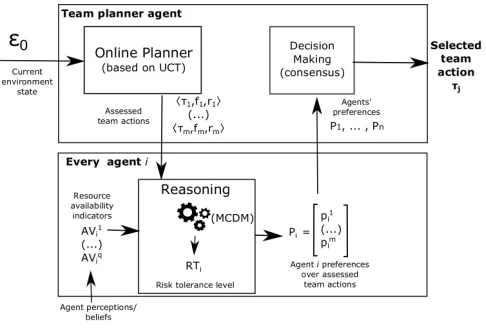
Fig. 2. Architecture of the risk-aware multi-agent planning framework
IV. RISK-AWAREONLINEMULTI-AGENTPLANNER
This section presents a novel multi-agent planning frame-work for collaborative, uncertain settings. The main contri-bution of the underlying online planning algorithm is the extension of the single-agent approach in [4] to assess risk of actions alongside their utility at team level. The proposed framework (depicted in Figure 2) is further combined with a collective MCDM approach for action selection at group level, as explained later in Section V.
A. Notation and Basic Concepts
The following notation is introduced to refer to the ele-ments utilised in the proposed planner. There exists a set AG = {1,2, . . . , n} of agents, and a finite action library
shared by all agents. Each actionak,1≤k≤m, is modeled
as a tuple hak, φk, effki. φk represents the preconditions for
the action to be applicable, witheffk ={(0, p)} the possible
(mutually exclusive) effects or outcomes 0 of the action at individual level, and their associated probabilityp. The set of all possible environment states is denoted byE, where0∈ E is the current state (root decision node in the search tree). The subset of all goal states is denoted byEG⊂ E. In the proposed
team planning approach, the team planner agent must manage information about multiple agents jointly, therefore it needs to formulate environment states at team level. Thus, a decision node is modeled upon the following two elements:
1) Agent-specific information about the state of every agent involved in the planning process, e.g. the current locations of robots in the nuclear scenario.
2) Other purely environmental information, e.g. the locations of unfixed targets (if any) in the nuclear site.
Based on this, a decision node associated to an environment state∈ Eis formalised as a 2-tupleD() =hs(AG);s(env)i, with s(AG) the current state of every agent and s(env) the environmental information.
Example 1:Consider the nuclear navigation scenario. The state s(i) of agent i is defined as a predicate of the form,
[image:3.612.94.261.51.274.2]in the execution of an action and is no longer available). Let s(env) = ∧at(target,L)L be the locations of targets (anomalies) not addressed yet. A decision node describing the state depicted in Figure 1 can be formalised as follows:
D() =h{at(1,0), at(2,6), at(3,15)}; 2∧3∧8∧9∧12i i.e. agents 1,2, and 3 are located respectively in zones 0,6,15. Furthermore, environmental information s(env)indicates the existence of untreated targets in locations 2,3,8,9,12.
Example 2:Letak be the action of moving from location0
to location 4 (i.e. crossing bridge12 upwards) in the nuclear scenario. Its corresponding formalisation is:
hmv 0 4, at(0),{(at(4),0.95),(at(−),0.05)}i The precondition for an agent to execute this action, φk =
at(0), is being situated in location0. The action has two pos-sible outcomes: (i) reaching location4, with95%probability; or (ii) failing to complete the action, with5% probability.
The representation of states and actions in our planning framework is based on PPDDL (Probabilistic Planning Do-main Definition Language) [20], which is fully compliant with implementations of approximate algorithms based on MCTS. We now introduce the concept of team action. This concept plays a central role in the proposed multi-agent planner.
Definition 1: A team action τ = {(i, ai
k), i ∈ pa(τ)}
encompasses a number of actions aik ∈ A simultaneously assigned to a team of agents pa(τ)⊆ AG (one action per agent). Team actions are formulated during planning, taking account of the current state and available actions per agent.
Example 3: Assuming the environment state represented in Figure 1, τ={(1, mv 0 4),(2, mv 6 7),(3, mv 15 14)} indicates that the robot1must move from 0 to 4, robot2must move from 6 to 7 and robot 3must move from 15 to 14.
B. Risk-Aware Online Team Planner
We now discuss how the online risk-aware planner intro-duced in [4] can be extended to deal with multiple collaborat-ing agents. To do this, we propose an online multi-agent plan-ner that (i) assesses both the risk and utility of actions from a team of agents, and (ii) returns a set of team actions with their associated utility and risk assessments, instead of returning a single best team action. We consider a MCTS-based search tree structure, with layers alternating between decision nodes,
D(), representing environment states , and chance nodes,
C(τ), representing team actionsτ. The children of a decision node reflect the team actions available at . Conversely, the children of a chance node indicate the stochastic outcomes or resulting environment states from applyingτ.
Below we describe how the outcomes of team actions and their probabilities of occurrence are determined. Having multiple agents executing a team action in parallel may involve a large number of possible outcomes, therefore we firstly discuss how the representation of such outcomes can be simplified, in order to prevent an excessive branching factor in the search tree. We assume two types of outcome for any τ:
success outcome,τ, whenallparticipating agents succeed in
completing their respective actions, and undesired outcome,
τ, otherwise. The undesired outcome of τ encompasses all
the possible eventualitiesF that may leadτ into failure (i.e.
one or more agents inpa(τ)failing to complete their assigned action). Therefore,τ =SF∈τF.
Importantly, the number of all possible undesired outcomes
F described byτ directly depends on the number of agents
participating in the team action,|pa(τ)|. Concretely, it is given by the number of possible subsets of agents, fa(τ)⊆pa(τ), that might succeed in completing their action, i.e. |τ| =
2|pa(τ)|−1. Both goal states
G ∈ EG (which result from
completing a sequence of team actions until reaching the goal established) and undesired outcomes τ ∈ EF (withEF ⊂ E
the set of all undesired outcomes) are terminal states, with ET =EG∪ EF the set of all terminal states.
Remark 1:A (summarised) undesired outcomeτis deemed
as a terminal state, because if an unexpected situation is encountered, the team planner agent starts another online planning process for the remaining agents upon the resulting environment state, taken as the new0.
Probabilistic information of individual actions must be combined to describe the effects of team actions. Let P(τ) be the probability of successfully completing τ, and P(τ) the probability of reaching any form of undesired outcome. Actions ak
i assigned to every agent i ∈ pa(τ) are regarded
as independent from each other, hence P(τ) can be easily calculated upon the individual action library information, as
P(τ) = Q
i∈pa(τ)P(aki), with P(aki) = p ∈ [0,1] being
the probability of reaching the expected (successful) effect of executing the agent actionaki =hak, φk,{(0, p),(0,1−p)}i.
Intuitively, P(τ) = 1−P(τ).
Below we introduce a reward function that allows for a reduced branching of the search tree by estimating a single reward value for all possible forms of undesired outcome.
Definition 2: LetET =EG∪ EF be the set of all terminal
states, as defined above. A reward function f is defined as a mappingf :ET →[−1,1]\{0}, with the following properties:
(i) f(G)>0,∀G∈ EG, i.e. arriving at a goal state always
produces a positive reward value.
(ii) f(τ) < 0, ∀τ ⊂ EF, i.e. arriving at any undesired
outcome always produces a negative reward value. (iii) Letd∈Nbe the depth level at which the terminal state
is encountered. Assume two identical terminal states1,
2 can be reached at depth d1 andd2 respectively, with
d1< d2. Thenf(1)≥f(2).
(iv) f(G)> f(τ)for anyG ∈ EG, τ ∈ EF.
According to (iii), a goal state is more rewarding when encountered after a lower number of team actions. Similarly, an undesired outcome is more detrimental when more effort is previously invested, i.e. after more actions. A discount factor
δ∈]0,1[is applied on f to reflect this property. The reward for an undesired outcome is calculated as follows:
f(τ) =−δd−1 P
F∈τPτ(F)·f(F)
P
F∈τPτ(F)
Clearly, f(τ) is calculated as the (discounted)
probability-weighted average of all possible forms of undesired outcome,
F ∈τ, which correspond to each of the non-empty subsets
fa(τ) of agents that fail to complete their associated action, such that fa(τ)∈ P(pa(τ))\{∅}. Their probability of occur-rence, denoted byPτ(F), is easily calculated upon individual
agent action information: Pτ(F) = Qi∈pa(τ)Pi(F), where
for each ak
i assigned to ithrough τ,
Pi(F) =
1−P(ak
i) if F at(i,−),
P(ak
i) otherwise.
(2)
The reward value for eachF is computed based on the amount
of failing agents in the team, i.e. f(F) = |fa
(τ)|
|pa(τ)|. This
non-negative value is only a partial step in the calculation of the overall negative reward for τ (Eq. (1)).
Since we consider a collaborative setting with a common goal pursued by all agents, the reward of a goal state is defined based on the discount factor δ and its depth d, as f(G) =
δd−1, i.e. the sooner the goal is accomplished (lower cost of executing actions), the more beneficial the outcome is.
Having defined the reward function, we now describe the procedure to assess risk, which extends the one in [4].
Definition 3: The immediate risk of taking a team actionτ
at state is the probability-weighted variance1 of its outcome
rewards:
IR(, τ) =P(τ)(f(τ)−E(, τ))2+P(τ)(f(τ)−E(, τ))2
(3) withE(, τ)the expected utility of takingτ at:
E(, τ) =P(τ)f(τ) +P(τ)f(τ) (4)
The success outcome of taking τ at is denoted byτ.
Eq. (1) allows to determine f(τ), but f(τ) can not be
directly calculated unless τ ∈ EG. Instead, reward values of
non-terminal states are calculated during the backpropagation phase. The immediate risk calculated by Eq. (3) is a measure associated to chance nodes (i.e. team actions). In decision nodes, however, the team of agents has a choice of which team action to execute. Therefore, we now define the immediate risk associated to a decision node.
Definition 4: Given a state and its set of immediately available team actions, Av(), the immediate risk exposure under a rational decision making perspective, is given by the immediate risk of the least risky team action available at :
RE() =minτ∈Av()IR(, τ) (5) The measure defined above considers the risk of immediate
team actions only, disregarding further actions beyond these, hence we modify it to assess an average cumulative risk upon the reward and immediate risk of courses of action.
Definition 5: The cumulative risk exposure at state is defined as:
CRE() =minτ∈Av()CM R(, τ) (6) 1Since we consider the use of approximate algorithms, the obtained
variances are in practice suitable approximations.
with CM R(, τ) the cumulative minimum risk of taking a team actionτ at, calculated as follows:
CM R(, τ) = IR(, τ) +CM Rold·visits(C(τ))
visits(C(τ)) + 1 (7)
visits(·)∈Nis the number of times a node has been visited. When a chance node is firstly visited,CM R(, τ) =IR(, τ). The selection and expansion phases are applied similarly to plain UCT, and multiple riskrolloutsare applied at each UCT iteration for resampling purposes, as explained in [4]. The
backpropagationphase is applied by updating both reward and risk estimated in an average cumulative fashion:
• The reward of a non-terminal state f() is updated every time D()is visited during backpropagation, tak-ing rewards of successive team action outcomes into consideration. Thus, f() is interpreted as the average cumulative reward of arriving at this state:
f() =f(
∗) +visits(N())·f old()
visits(N()) + 1 (8) Here, f(∗) is the reward of the expected (success) outcome of the least risky action inAv().
• The updated risk estimate of a chance node in the backpropogation path is compared to that of its sibling nodes, and the risk of the sibling chance node with lowest risk estimated at that level is backpropagated.
The planner finally returns (a subset2 of) team actions with their associated risk and reward estimates, rather than a single, most rewarding team action. Theseassessed team actionsare subsequently evaluated by participating agents (Section V).
The following example illustrates the calculation and back-propagation of reward and risk estimates back to the root node.
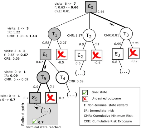
Example 4: Consider the search tree excerpt depicted in Figure 3, where the nodes corresponding to τ5 and its out-comes have been newly expanded. As a result of a roll-out, a goal state with reward f(G) = 0.7 is encountered.
This reward is backpropagated straightaway up to the last decision node generated, N(5). The immediate risk of the predecessor chance node, C(τ5), is calculated (Eq. (3)), re-sulting in IR(1, τ5) = 0.09. Since this is the first time
C(τ5) is visited, its cumulative minimum risk is trivially
CM R(1, τ5) =IR(1, τ5) = 0.09. This value is compared to that of its existing sibling node so far, and it is lower than
CM R(1, τ4) = 0.59, it is backpropagated as the cumulated risk exposure at 1, CRE(1) = 0.09. The reward at this state is updated (Eq. (8)) based on its previous reward, the reward being backpropagated, and the visit count, resulting in f(1) = (0.65·2 + 0.7·1)/3 = 0.67. The chance node
C(τ1)has been previously visited, hence both the immediate and cumulative minimum risk ofτ1are updated by using Eqs. (3) and (7), respectively. By comparingCM R(τ1) with that of its sibling nodes, CM R(τ3) < CM R(τ1), therefore the estimates in the parent node,f(0),CRE(0), are updated by backpropagating estimates fromτ3(instead ofτ1) in this case. 2If the number of immediately available team actions is large, those ones
Fig. 3. Reward calculation and backpropagation (see Example 4)
V. RISK-AWAREMULTI-AGENTDECISIONMAKING
This section describes the multi-criteria group decision making approach applied by agents to jointly select one of the candidate team actions returned by the planner. Firstly, risk attitude-based reasoning process conducted by agents to assess the available team actions. A GDM procedure is then undertaken to collectively select the best team action.
A. Preference Modeling upon Multiple Criteria
In order to rationally evaluate team actions, every agent
i needs to determine its risk tolerance level RTi ∈ [0,1],
calculated based on the availability ofq≥1resources deemed as relevant by i. Resource availability determines the attitude the agent should adopt towards risk, and the availability of each resource is viewed as the satisfaction degree of a criterion, under an MCDM perspective. RTi is computed by
using a functionρithat aggregates resource availability levels:
RTi=ρi(AVi1, . . . , AV q
i ) (9)
Each argumentAVk
i ∈[0,1],k∈1. . . q, is an availability
indicator of thek-th resource: the larger its value, the higher the availability. Moreover, from the non-decreasing property fulfilled byρi, the higher any of theAVik is, the closerRTiis
to one, hence the more tolerant agentiis towards risky actions. The aggregation function ρi can be customised to suit each
specific scenario and agent, by establishing the resource levels relevant to each agent and the way its associated indicators are determined. This allows agents to flexibly consider different (sets of) resources when calculating RTi.
Example 5: Consider the nuclear navigation scenario. An agent i utilises the following four availability indicators to assess its risk tolerance level: AV1
i , remaining battery life;
AV2
i : remaining time;AVi3, number of agents still operating;
AV4
i , number of anomalies addressed in the nuclear plant so
far. In order to express these indicators as values in [0,1],
they can be easily defined as percentages with respect to a full battery level, the total available time, number of agents in the team and anomalies initially detected, respectively.
Examples of aggregation functions that can be utilised byi
to aggregate availability levels intoRTiinclude: (i) arithmetic
mean; (ii) weighted mean; or (iii) the Ordered Weighted Averaging (OWA) operator [21], in which elements are firstly arranged in decreasing order, and importance weights W =
{w1, . . . , wq} (Pkwk= 1) are assigned to ordered elements.
OWA operators allow to reflect different optimistic (resp.
pessimistic) attitudes in the aggregation process, depending on importance weights being rather assigned to the highest or lowest elements to aggregate. Yager defined an measure of optimism,OW ∈[0,1], to categorise OWA operators [22]:
OW = Pq
k=1(q−k)wk
q−1 (10) Optimistic (OR-like) OWA operators accomplish OW >0.5.
Conversely, pessimistic (AND-like) operators fulfill OW <
0.5, and neutral operators fulfillOW = 0.5.
Example 6: Consider agent i from the previous example. Assume its remaining battery life is 70% (AV1
i = 0.7), half
of the time limit elapsed (AV2
i = 0.5), all agents still operate
(AV3
i = 1) and two out of five anomalies have been dealt with
(AV4
i = 0.4). The agent utilises the OWA operator to calculate
RTi, by adopting a slightly optimistic, OR-like aggregation
attitude [21] given by the vectorW ={0.3,0.3,0.2,0.2}:
RTi=1·0.3 +0.7·0.3 +0.5·0.2 +0.4·0.2 = 0.69
Notice that the optimistic attitude stems from larger impor-tance weights being associated to the two largest arguments, 1 and0.7. Furthermore,OW = 0.566>0.5.
Given RTi and the m assessed team actions hτj, fj, rji
returned by the online planner, j = 1, . . . , m, each agent proceeds to construct a preference vectorPi= [p1i p2i . . . pmi ],
where a rating pji ∈ [0,1] indicates its satisfaction degree with τj: the higher p
j
i, the more satisfied i is with τj. The
assessed reward fj, assessed risk rj, and the agent attitude
towards risk are three determinant criteria to compute a rating for each team action. Therefore,pji is calculated as a function
π: [0,1]×[0,1]×R→[0,1]of such criteria:
pji =π(RTi, fj, rj)
withπaccomplishing the following three properties:
i. If RTi > 0.5 the agent adopts a risk tolerant attitude,
tending to favor team actions with higher reward. ii. If RTi < 0.5 the agent adopts a risk averse attitude,
tending to favor team actions with lower risk.
iii. If RTi = 0.5 the agent has a risk neutral attitude,
deeming reward and risk of team actions as equally important criteria.
agent risk tolerance level. This results in deriving a preference degree that appropriately balances utility and risk:
pji =RTi·fj+ (1−RTi)·(1−rj) (11)
Before applying Eq. (11), the assessed reward and risk of
τj are normalised to take values in the unit interval:
fj =
fj−minkfk
maxkfk−minkfk
rj=
rj−minkrk
maxkrk−minkrk
(12) with k ∈ {1, . . . , m}. Normalisation implies that for the assessed team action with highest (resp. lowest) reward, we havefj = 1 (resp.fj = 0). Similarly, for the most and least risky assessed team actions, rj= 1 andrj= 0, respectively.
Example 7:ConsiderRTi= 0.69from the previous
exam-ple (iis slightly inclined towards rewarding team actions rather than low risk ones), and the following assessed team actions returned by the planner, hτ1,0.43,1.08i, hτ2,−0.07,0.36i, hτ3,0.83,1.45i,hτ4,0.3,1.15i. Its associated preference vector is Pi = [0.56 0.31 0.69 0.51]. The slightly risk tolerant
attitude is reflected through the agent preference towards higher rewards, as occurs withτ3 for instance.
B. GDM Approach for Team Action Selection
All active agents provide their preferences Pi to the team
planner agent, which elicits them and defines a GDM problem on{P1, . . . , Pn}aimed at making a common accepted solution
on the next team action to undertake. Concretely, an aggre-gated team preferencePcthat minimises the distance between
individual preferences of agents and Pc, i.e. a consensus
preference, is sought [12]. An automatic, iterative consensus-reaching approach is conducted, by applying the optimal preference aggregation method proposed by Lee in [23].
Letd(Pi, Ph)∈[0, m]denote the dissimilarity between two
preference vectors Pi,Ph, computed by using a Minkowski
distance measure d, e.g. the Euclidean distance, given by:
d(Pi, Ph) = v u u t
m X
j=1
(pji−pjh)2 (13)
An approximation to an optimal team preference vector
Pc = [p1c, . . . , pmc ] that minimises the sum of (weighted)
dissimilarities with individual preferences can be obtained by an iterative algorithm similar to Fuzzy C-means [23]. The algorithm weighs the preferences of agents assuming every agent preference Pi is initially regarded as equally important,
assigning wi= 1/n,∀i∈ {1, . . . , n}
pjc = P
i(wi)µp j i
(wi)µ
wi=
(1/d(Pi, Pc))
1/(µ−1)
P
l(1/d(Pl, Pc))
1/(µ−1) (14)
This process is iteratively applied, for each pjc ∈ Pc and
wi∈W respectively, until satisfying a stopping condition, e.g.
when weights of agents preferences stabilise, i.e. kW(t+1)−
W(t)k ≤κ, witht andt+ 1 two iterations of the consensus-reaching algorithm, andκ≈0,κ >0the threshold difference
used as stopping criterion. The parameter µ ≥ 1 is utilised to control the influence of noisy information, i.e. agents preferences whose weight is low due to their preferences being situated far from consensus, compared to that of preferences with largerwi: the largerµ, the stronger the difference between
the influence made by agents positioned close and far from consensus. The convergence of the algorithm is thoroughly demonstrated in [23]. The resulting collective preferencePc is
utilised to select the best3 team actionτ∗ withp∗i = maxjpjc,
as the “best” (most preferred) team action for its execution. This team action is finally executed by agents inpa(τ∗).
VI. EXPERIMENTS ANDRESULTS
In this section we demonstrate the performance of the proposed multi-agent planning framework. Throughout exper-iments, we refer to the nuclear navigation scenario (Section III, Figure 1) with three robots and five target anomalies.
We start by evaluating the overall performance of the framework by comparing it against threebaselineapproaches:
B1: Risk-aware planning, individual decision making: Instead of making a collective decision, only the team planner agent evaluates candidate team actions by balancing re-ward and risk (based on its own attitude tore-wards risk). B2: Risk-aware planning, lowest-risk team action selection:
The team planner agent directly selects the lowest-risk available team action, i.e. without balancing reward and risk.
B3: Reward-driven planning: Only the reward of team ac-tions is assessed during planning (risk is not assessed), therefore the immediate team action with highest reward estimate is returned by the planner straightaway, with no need for subsequent decision making process.
10 different settings are considered for the (success) proba-bilities of agent actions, ranging betweenpw∈[0.86,0.95]for
crossing wider bridges, and withpn =pw−0.05for narrower
bridges. The experiments were run 100 times, gathering the following two metrics:
• Success Rate(%): Number of executions where the goal
of completing the five targets is achieved beforeallthree robots fall off a bridge.
• Average Reward when Successful: Average reward f
associated to the result of successful executions. To this end we calculate the reward of an outcome reached upon execution of actions, after which some agents might have failed. According to this, the f(G) calculated during
planning is adjusted by multiplying it by the proportion of “surviving” agents,#surv/3. This metric provides an estimate of the cost invested in reaching the goal. Figure 4 shows the results obtained for each metric and action probability setting. In general, balancing the reward and potential risk of team actions leads to higher chances of success. This becomes more noticeable as the success probabilities of agent actions decrease. The difference in
3Bestis understood in this context as the most collectively accepted team
pw pw
Fig. 4. Success rate (left) and average reward when successful (right) of the proposed risk-aware framework against three baseline approaches.
performance accentuates when compared with (B3), i.e. when the team planning process is purely reward-driven and risk is completely ignored. Results demonstrate that assessing risk alongside reward of team actions, and making more informed, context-aware decisions based on all agents’ viewpoints to-wards risk, becomes increasingly beneficial in cooperative settings, particularly as the uncertainty of action effects in-creases. On the contrary, relying on only one agent to make decisions (B1) does not provide optimal results in multi-agent settings, thus the need for rational collective decision making mechanisms among agents is justified.
A larger average reward when successful is generally ob-served with the proposed risk-aware framework regardless of the agent action probabilities. Only in some cases the reward-driven baseline (B3) slightly outperforms in average reward, however this occurs at the cost of a much lower % success with respect to the other approaches being compared (as outlined above). The lowest-risk approach (B2) shows the most accentuated difference with our framework in terms of average reward when successful. Overall, results show that the cost of reaching the goal can be reduced when planning and making decisions predicated on risk assessment.
VII. CONCLUDINGREMARKS
This work presented a collaborative multi-agent planning framework for domains where agent actions have uncertain effects, that integrates an online multi-agent planner capable of assessing risk alongside utility of actions, with a multi-criteria group decision making approach that enables the collective selection of an accepted solution for the planing problem. As a result, agents make rational decisions by balancing the risk and utility of actions based on their attitude towards risk. Future work aims at extensions to larger-scale scenarios through subgroup delegation and uncertain information fusion.
ACKNOWLEDGMENTS
This work has been funded by EPSRC PACES project (Ref: EP/J012149/1).
REFERENCES
[1] D. Weld, “Recent advances in AI planning,”AI Magazine, vol. 20, pp. 93–123, 1999.
[2] M. de Weerdt and B. Clement, “Introduction to planning in multiagent systems,”Multiagent Grid Syst., vol. 5, no. 4, pp. 345–355, 2009.
[3] A. Torre˜no, O. Sapena, and E. Onaindia, “Global heuristics for dis-tributed cooperative multi-agent planning,” inProc. ICAPS 2015. AAAI Press, 2015, pp. 225–233.
[4] R. Killough, K. Bauters, K. McAreavey, W. Liu, and J. Hong, “Risk-aware planning in BDI agents,” inProc. ICAART’16, 2016.
[5] B. Abramson, “The expected-outcome model of two-player games,” Columbia University, Tech. Rep. CUCS-315-87, 1987, ph.D. Thesis. [6] T. Keller and P. Eyerich, “PROST: Probabilistic planning based on
UCT,” inProc. ICAPS’12, 2012.
[7] F. Wu, S. Zilberstein, and X. Chen, “Online planning for ad hoc autonomous agent teams,” inProc. IJCAI 2011, 2011, pp. 439–445. [8] ——, “Online planning for multi-agent systems with bounded
commu-nication,”Artificial Intelligence, vol. 175, no. 2, pp. 487 – 511, 2011. [9] F. S. Melo and A. Sardinha, “Ad hoc teamwork by learning teammates’
task,”Autonomous Agents and Multi-Agent Systems, vol. 30, no. 2, pp. 175–219, 2015.
[10] M. Doumpos and E. Grigoroudis,Multicriteria Decision Aid and Arti-ficial Intelligence. Wiley, 2013.
[11] J. Lu, G. Zhang, D. Ruan, and F. Wu,Multi-Objective Group Decision Making. Imperial College Press, 2006.
[12] I. Palomares, F. Estrella, L. Mart´ınez, and F. Herrera, “Consensus under a fuzzy context: Taxonomy, analysis framework AFRYCA and experimental case of study,”Information Fusion, vol. 20, no. November 2014, pp. 252–271, 2014.
[13] L. Kocsis and C. Szepesv´ari, “Bandit based monte-carlo planning,” in Proc. ECML’06, 2006, pp. 282–293.
[14] C. Browne, E. Powley, D. Whitehouse, S. Lucas, P. I. Cowling, P. Rohlfshagen, S. Tavener, D. Perez, S. Samothrakis, and S. Colton, “A Survey of Monte Carlo Tree Search Methods,”IEEE Transactions on Computational Intelligence and AI in Games, vol. 4, no. 1, pp. 1–43, March 2012.
[15] P. Delias and N. Matsatsinis,Multicriteria Decision Aid and Artificial Intelligence. Wiley, 2013, ch. Multiple criteria decision aid and agents: Supporting effective resource federation in virtual organizations. [16] B. Roy,Multicriteria Methodology for Decision Aiding. Dordrecht:
Kluwer, 1996.
[17] G. Beliakov, A. Pradera, and T. Calvo,Aggregation Functions: A Guide for Practitioners. Springer, 2007.
[18] M. Detyniecki, “Fundamentals on aggregation operators,”LIP6 Research Report:2001-2002, University of California, Berkeley, 2001.
[19] S. Saint and J. R. Lawson,Rules for Reaching Consensus. A Modern Approach to Decision Making. Jossey-Bass, 1994.
[20] H. Younes and M. Littman, “PPDDL1.0: An extension to PDDL for expressing planning domains with probabilistic effects,” in Proc. ICAPS’03, 2003.
[21] R. Yager, “On ordered weighted averaging aggregation operators in multi-criteria decision making,” IEEE Transactions on Systems, Man and Cybernetics, vol. 18, no. 1, pp. 183–190, 1988.
[22] A. Kishor, A. K. Singh, and N. R. Pal, “Orness measure of owa operators: A new approach,” IEEE Transactions on Fuzzy Systems, vol. 22, no. 4, pp. 1039–1045, 2014.