Towards improving numerical weather predictions by evolutionary computing techniques

Procedia Computer Science 9 ( 2012 ) 1056 – 1063

1877-0509 © 2012 Published by Elsevier Ltd. doi: 10.1016/j.procs.2012.04.114

International Conference on Computational Science, ICCS 2012

Towards Improving Numerical Weather Predictions by

Evolutionary Computing Techniques

$

Hisham Ihshaish1,∗, Ana Cort´es, Miquel A. Senar

Departament d’Arquitectura de Computadors i Sistemes Operatius, Escola d’Enginyeria, Universitat Aut`onoma de Barcelona, 08193 Bellaterra (Barcelona), Spain

Abstract

Weather forecasting is complex and not always accurate, moreover, it is generally defined by its very nature as a process that has to deal with uncertainties. In a previous work, a new weather prediction scheme was presented, which uses evolutionary computing methods, particularly, Genetic Algorithms in order to find the most timely ‘optimal’ values of model closure parameters that appear in physical parametrization schemes which are coupled with numerical weather prediction (NWP) models. Currently, these parameters are specified manually. Our hypothesis is that the NWP model forecast skill is sensitive to the specified parameter values. And thus, by finding ‘optimal’ values of these parameters, we aim to enhance prediction quality. In this work however, the same scheme is extended by introducing different ways of prediction evaluation during the process of searching closure parameter values. To verify our new scheme, we show prediction results of an experimental case using historical data of a well known weather catastrophe: Hurricane Katrina that occurred in 2005 in the Gulf of Mexico. Obtained results provide significant enhancement in weather prediction.

Keywords: numerical weather prediction; evolutionary computing; ensemble prediction; parameter estimation

1. Introduction

Numerical weather prediction (NWP) models, as well as the atmosphere itself, can be viewed as nonlinear dynam-ical systems in which the evolution depends sensitively on the initial conditions. Moreover, weather prediction is, by its very nature, a process that has to deal with uncertainties. The initial conditions of a NWP model can be estimated only within a certain accuracy. During a forecast, some of these initial errors can be amplified and result in significant forecast errors.

$_{This research has been supported by the MICINN-Spain under contract TIN 2007-64974.}

∗_{Corresponding author:}

Email address:hisham ihshaish@caos uab es(Hisham Ihshaish)

Besides initial-condition error, weather and climate prediction models are also sensitive to errors associated with the model itself. In particular, the uncertainty due to the parameterizations of sub-grid-scale physical processes is known to play a crucial role in prediction quality (e.g., [1]). Prediction errors caused by the uncertainty in physical parameterizations is commonly referred to as model errors. Being that said, weather predictability errors are normally subject to two kinds of errors, initial condition errors and model errors.

By figuring out the main sources of error in predictability of NWP models, many efforts had been focusing on enhancing prediction quality, mainly on developing sophisticated and skillful next-generation NWP models (e.g., [2] and [3]), addressing the uncertainty of initial conditions by better estimation techniques, and also on developing physical parametrization models or schemes which are nowadays coupled with NWP models and lead to improved predictive skill.

Over the past 20 years or so, stochastic or ”ensemble” forecasting [4] became a practical and successful way of addressing the predictability problem associated with the uncertainty in initial conditions. Ensemble forecasting is conducted by better estimations of the atmospheric initial state (initial conditions) which is produced by data assimi-lation (DA)[5] techniques, and then, initial state perturbations are computed and launched in different forecasts, each is initiated by a perturbed initial state. Early on moreover, several weather prediction centers have addressed this problem by developing operational ensemble prediction systems (EPS) (e.g., [6]). The Ensemble spread finally, is used to indicate forecast uncertainty. However, and although it has been realized that there is a stochastic nature of physical parameterizations in ensemble prediction (predictability is sensitive to variations in physical parameters), it has not been straightforward to develop theoretically sound, and also practical, formulations for how to insert param-eterization uncertainty into ensemble development [7, 8].

On the other hand, and in contrast to the dynamics of NWP models, which are based on fundamental physical concepts, physical parameterizations, although partly are based on fundamental concepts of physics, involve empirical functions and tunable parameters, which usually referred to as model closure parameters. Practically, all physical parametrization schemes contain closure parameters and typically, expert knowledge and manual techniques are used to define the optimal parameter values, based on observations, process studies, large eddy simulations, etc. Therefore, some parameter value combinations score better than others, but it is very demanding to manually specify the optimal combination.

In [9], it was shown how forecast skill is sensitive to a set of these closure parameters, and moreover, a prediction scheme (G-Ensemble) that uses Genetic Algorithm (GA), to estimate ‘optimal’ values for these parameters for a cer-tain forecast, in order to enhance forecast skill was presented. The proposed scheme showed significant enhancement in prediction quality, and thus, we extend in this paper our proposal by a different implementation for forecast skill calculation when evaluating the score of a set of parameter value combinations.

The rest of the paper is organized as follows: Section 2 gives a brief description of our previous work (G-Ensemble

scheme) for closure parameter estimation in NWP models. In section 3, the extended version of the G-Ensemble

scheme is presented and described. Section 4 discusses experimental results obtained with a test case. Finally, conclusions and future work are described in section 5.

2. G-Ensemble

In this section, our Genetic Ensemble (G-Ensemble) approach [9] for prediction enhancement is briefly described, as well as the set of the model closure parameters targeted for better estimation. The main objective of the presented scheme is to enhance prediction quality by better estimating a set of NWP model closure parameters. Our study focuses on finding optimal values ofLanduseandSoilclosure parameter (the land surface parameters and the impact they have are described in [10]). The optimization of these parameters will serve as a prove of concept of our method, which could be applied to other parameters. These parameters are found in land surface physical schemes (LSM) (e.g.,[11, 12]) which are coupled to most NWP models.

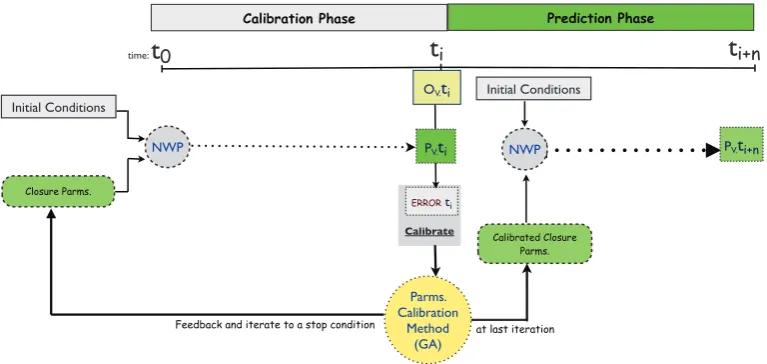
Calibrate

Prediction Phase Calibration Phase

time:

t

t

t

ERROR ti

NWP NWP

Initial Conditions

Feedback and iterate to a stop condition

PV.ti+n

Closure Parms.

PV.ti

Parms. Calibration

Method (GA)

Calibrated Closure Parms.

OV.ti Initial Conditions

at last iteration

Figure 1: Two-phase prediction scheme; NWP is the a numerical weather prediction model. tiis time 00:00 of prediction process,

t0is a time instant previous to Prediction Phase (initial time of Calibration Phase), ti+nis the future time to be predicted.”OV”is

an observed meteorological variable at time ti,”PV”is the predicted variable at the same time using a NWP model.

The process of closure parameter estimation in Calibration Phase proceeds as follows:

(i) at the beginning of Calibration Phase (time t0 in Fig. (1): a sample of the targeted parameter values from ensemble proposal distribution is generated (perturbations in closure parameter values);

(ii) the generated parameter values are inserted to the ensemble prediction model;

(iii) an ensemble of forecasts (the prediction model is different for each ensemble member regarding the targeted parameter values), is conducted to predict meteorological variables at timeti, where real observations are avail-able;

(iv) evaluation of a fitness function for each ensemble member is done at timeti;

(v) genetic algorithm functions (selection, crossover and mutation) are used to generate a new ensemble distribution from the set of combinations of closure parameters which score better predicting at timeti; and

(vi) the process is repeated iteratively until an acceptable error value, or a predefined number of iterations is achieved.

The used fitness function depends on the number of meteorological variables to be better predicted, as such, if

theG-Ensembleis used to enhance prediction for one single meteorological variable, we use the root mean square

error (RMS E) as the the fitness function for the GA to be minimized. This approach is referred to asSingle-Variable

G-Ensemble. In contrast, as it is necessary to enhance prediction for a set of meteorological variables, the normalized

root mean square error (NRMS E) is used as the fitness function to be minimized during Calibration Phase, (see equation (1)). This approach is calledMulti-Variable G-Ensemble.

NRMS E=

_n

i=1(xobs,i−xpre,i)2

n

xobs(max)−xobs(min)

(1)

InNRMS Eequation,xobsis an observed value of a variablexandxpreis the predicted value for the same variable.

For example, the NRMS E of an ensemble member that predicts Temperature (T) and Precipitation (P) is the percentage obtained by the summation of two percentages: NRMS E(T) andNRMS E(P), as shown in equation (2).

Error=NRMS E(var1)+NRMS E(var2)=value% (2)

In spite of the fact that the objective in our scheme is to minimize theRMS EorNRMS Ein Calibration Phase, as the fitness function used for the evaluation of ensemble members, other fitness functions are applicable to be used in the presented scheme. The GA could be oriented to minimize any other targeted fitness functions.

At the last iteration in the Calibration Phase, the values of closure parameters, which produced the least value of

RMS E orNRMS E, i.e. the ensemble member with the best forecast skill score at timeti, is selected to be used in

Prediction Phase. This ensemble member is called: Best Genetic Ensemble Member (BeGE M). Our hypothesis was that, for short-range weather forecasts, if the forecast skill is improved in the Calibrations Phase by a set of a calibrated closure parameters, then, the same closure parameter values will also improve forecast skill during Prediction Phase.

By now, in Prediction Phase, a deterministic forecast is used in our experiments, in other words, theBeGE M

which is the ensemble member having the calibrated closure parameter values is the single forecast to be conducted in Prediction Phase. However, the producedBeGE Mcould be integrated in any type of EPS considering perturbations in initial conditions during Prediction Phase.

3. Extended G-Ensemble

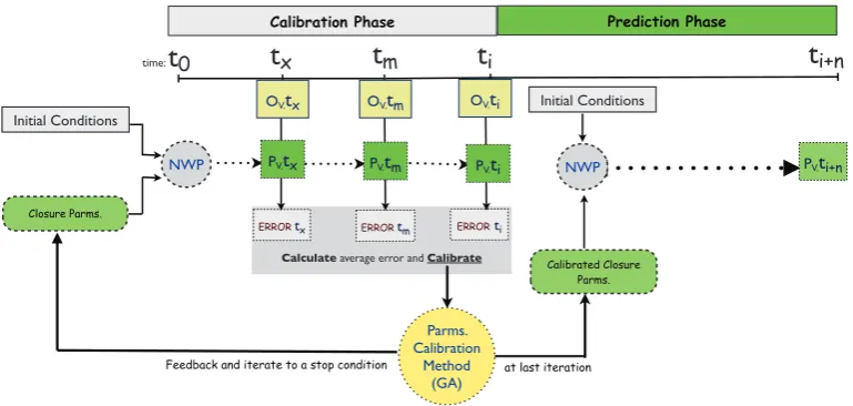
In this section, an extended version of theG-Ensembleapproach is presented. Precisely, the main change is done in the Calibration Phase, as such, it is supposed that evaluating ensemble members during Calibration Phase according to one single observation for each meteorological variable is not that fair, basically, due to the stochastic nature of NWP ensembles, some ensemble members may change their performance over time. Hence, to help the used GA to take better decisions when selecting the set of ensemble members that will reproduce a consecutive generation of ensemble members in each iteration, G-Ensemblescheme is extended such that it becomes capable to evaluate ensemble members according to a window of observations rather than ‘one-point’ observation.

Back to Fig.(1), ensemble members are evaluated according to real observations available atti. In contrast, the extended version of ourG-Ensemble(shown in Fig. (2)), ensemble members are evaluated according to observations available in more than one point during Calibration Phase.

Calculate average error and Calibrate

Prediction Phase Calibration Phase

time:

t

t

t

ERROR ti

NWP NWP

Initial Conditions

Feedback and iterate to a stop condition

PV.ti+n

Closure Parms.

ERROR tx

t

t

ERROR tm

PV.ti

PV.tx PV.tm

Parms. Calibration

Method (GA)

Calibrated Closure Parms. OV.tm

OV.tx OV.ti Initial Conditions

at last iteration

Figure 2: Extended Two-phase prediction scheme; NWP is the a numerical weather prediction model. tiis time 00:00 of prediction

process, t0is a time instant previous to Prediction Phase (initial time of Calibration Phase), ti+nis the future time to be predicted,

tx and tm are time instants within the Calibration phase where real observations are available as in ti. ”OV”is an observed

If prediction is needed to take place from timetitoti+n, Calibration Phase is to be conducted in the interval (t0-ti), however, observations could be available at timestx,tm(any model time steps that fall within Calibration Phase), as well as at timeti. Being these observations available, the GA fitness function considers the average error of the three error values calculated at timestx,tmandti, for each ensemble member according to the three observations available at the same time instants.

The same process is done for Calibration and Prediction as described in the pervious section, however, theBeGE M

in the Calibration Phase of the extended version of theG-Ensembleis produced by evaluating its forecast skill accord-ing to a window of observations rather than a ‘one-point’ observation.

In the next section, experimental results are discussed to verify prediction enhancement gained by the proposed extendedG-Ensemblescheme.

4. Experimental Evaluation

To test our approach, we used historical data of hurricane Katrina[13], which occurred on August 28, 2005 in the Gulf of Mexico and unfortunately caused the death of more than 1,800 persons along with a total property damage that was estimated at $81 billion (2005 USD). The objective of the experiments is to predict meteorological variables evolution from time: 12:00 h. of the day 28/08/2005 to time 00:00 h. of 30/8/2005 (a period of 36 hours in which the major effects of the hurricane were produced). The model is configured to predict the evolution of meteorological variables each one hour and the spatial resolution of the domain was 12km. The used NWP model in our experiments was the Weather Research and Forecasting (WRF) [2] and all Physics schemes were the same for all experiments.

To get the evolution of meteorological variables at 12:00 h. of 28/08/2005, we used initial conditions of the atmospheric state in the zone three hours before, i.e. model started prediction from time 09:00 of 28/08/2005. For our approach (G-Ensemble), the Calibration Phase started from time 00:00 of 28/08/2005 to time 09:00 of the same day. The variables predicted in our experiments were:Latent Heat Flux LHF (W/m2),2-meter Temperature (◦C), and the

Accumulated Precipitation RAINC (mm).

In the subsequent experiments, prediction errors (RMS EandNRMS E) produced during Prediction Phase of three ways of prediction are compared;

(a) G-Ensembleapproach, where Calibration considers ‘one-point’ observation, at time 09:00 of 28/08/2005

(BeGE M(1−point))

(b) G-Ensembleextended approach, where Calibration considers a window of observations, at time 7:00, 8:00 and

09:00 of 28/08/2005 (BeGE M(window)).

(c) The EPS, which is useed to refer to the average error of an ensemble forecast conducted by the initial ensemble members used in the first iteration of Calibration Phase (an ensemble forecast such that the prediction model is different for each ensemble member regarding the targeted parameter values, these variables are not calibrated).

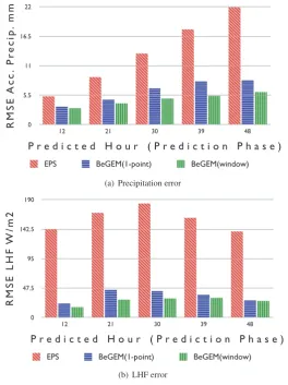
It should be mentioned, however, that all the subsequent results represent the average of a set of executions. This is done to assure that the obtained results are reliable by avoiding the randomity which could be produced in GA operations in some cases. Firstly, we show experimental results for two different cases: to predict Accumulated Precipitation (results shown in Fig.5(a)) and to predict Latent Heat Flux (results shown in Fig.5(b)).

The Genetic Algorithm of the Calibration Phase was configured to iterate 15 times over an initial population size of 40 individuals (initial ensemble size). Its three main operators were configured as follows:Selection: (best one of two) and (roulette),Crossover: (probability=0.7, type: two points crossover), andMutation: (probability= 0.2).

In both cases, with the same initial ensemble members used in the EPS case, a significant improvement in predic-tion quality obtained by theG-Ensembleapproach over the EPS. Additionally, it could be also observed that better enhancements in predictions were obtained by the extendedG-Ensembleapproach.

The extendedG-Ensembleapproach is also used to enhance predictions of a set of meteorological variables at the same time, by applying theMulti-Variable G-Ensembleand using the errorNRMS Ein Calibration Phase as the fitness function of the GA. In this case, significant improvements in the prediction of a set of meteorological variables at the same time were also obtained. Fig.(4) shows the results obtained in this case. Again, significant reduction of

theNRMS Ewas obtained in the prediction of a set of meteorological variables together and, the extended version of

0 5.5 11 16.5 22

12 21 30 39 48

RMSE

Acc

. Pr

ecip

. mm

P r e d i c t e d H o u r ( P r e d i c t i o n P h a s e )

EPS BeGEM(1-point) BeGEM(window)

(a) Precipitation error

0 47.5 95 142.5 190

12 21 30 39 48

RMSE LHF

W/m2

P r e d i c t e d H o u r ( P r e d i c t i o n P h a s e )

EPS BeGEM(1-point) BeGEM(window)

(b) LHF error

Figure 3: Single-Variable G-Ensemble ; (a): RMS E error in prediction of variable Acc. Precipitation and (b): variable LHF. Results are of classical EPS, BeGEM(1-point) and BeGEM(window) for both variables.

0 0.5 1

12 21 30 39 48

NRMSE ERR

OR

P r e d i c t e d H o u r ( P r e d i c t i o n P h a s e )

EPS BeGEM (1-point) BeGEM (window)

Additionally, it is observed that the reduction in theNRMS Eof the three variables together, also provides an en-hancement in the prediction of each meteorological variable alone. In other words, all variables were better predicted

whenG-Ensembleoriented to reduce theNRMS Eof those variables together. To illustrate these results, Fig.(5) shows

how the corresponding prediction error of each variable was reduced whenG-Ensemblewas oriented to reduce the

NRMS Eof the three variables together.

0 6 11 17 22

12 21 30 39 48

RMSE Acc

.Pr

ec

.

mm

P r e d i c t e d H o u r

EPS BeGEM(1-point) BeGEM(window)

(a) Precipitation RMSE

10 58 105 153 200

12 21 30 39 48

RMSE LHF mmW/m2

P r e d i c t e d H o u r

EPS BeGEM(1-point) BeGEM(window)

(b) LHF RMSE

0 1 2 3 4

12 21 30 39 48

RMSE T2

Cº

P r e d i c t e d H o u r

EPS BeGEM(1-point) BeGEM(window)

(c) 2-m Temperature RMSE

Figure 5: RMS E prediction error of: (a) Accumulated Precipitation RAINC, (b) Latent Heat Flux LHF), and (c) 2-meter Tem-perature. Prediction using BeGEM (1-point) and BeGEM (window) produced after 15 iterations of the Calibration Phase of the Multi-Variable G-Ensemble.

Finally, it was shown in [9] that the proposedG-Ensembleapproach is cost effective computationally compared to the classical EPS over a parallel computing environment, many execution scenarios were tested over a cluster of 30 computing nodes, and the prediction quality was significantly enhanced, whereas, execution time was reduced in comparison with a classical EPS run in Prediction Phase. Besides, in the extendedG-Ensemble, no new computations are introduced; fitness evaluation over more than one point is not computing intensive; that is, it involves simple mathematical operations to calculate the average error regarding various observations.

5. Conclusions and future work

This work describes our ongoing investigation mainly focused on enhancing short-range weather forecasting by estimating optimal NWP model closure parameter values, using an evolutionary computing method; genetic algo-rithm. In [9], it is shown how forecast skill is sensitive to model closure parameter values, moreover,G-Ensemble

prediction scheme is presented, which aggregates a Calibration Phase to the prediction process, where these parameter values are optimized to improve forecast skill. TheG-Ensembleprediction scheme showed a significant improvement in prediction quality.

In this paper,G-Ensembleis extended in a way in order to consider more than observation point in the evaluation of forecasts during Calibration Phase. This addition enables the genetic algorithm which is used during Calibration Phase, to make better decisions when selecting between forecasts through its iterations. By introducing this capability to our scheme, it was shown by experiments, that forecast skill is improved while no computational cost is added.

Both theG-Ensembleand the presented extension, could be integrated in any operational EPS, that is, the produced

BeGEMwith the calibrated closure parameters could be considered as a well-tuned model regarding its closure

pa-rameters. Hence, for a certain forecast to be conducted using an EPS (considering perturbations in initial conditions),

BeGEMprovides a ‘physics’ well-tuned model to maximize EPS prediction quality.

These results encourage us to continue our research efforts by testing our scheme over larger sets of model clo-sure parameters, as well, we are planning to design methods that handle real observations during prediction process deciding their injection intervals at run-time in order to get more reliable meteorological predictions.

References

[1] T. N. Palmer, A nonlinear dynamical perspective on model error: A proposal for non-local stochastic-dynamic parametrization in weather and climate prediction models, Quarterly Journal of the Royal Meteorological Society 127 (572) (2001) 279–304.

[2] Weather Research and Forecasting Model homepage. URLhttp://www.wrf-model.org/index.php

[3] PSU/NCAR MM5 community model homepage. URLhttp://www.mmm.ucar.edu/mm5/

[4] M. Leutbecher, T. N. Palmer, Ensemble forecasting, J. Comput. Phys. 227 (2008) 3515–3539. doi:10.1016/j.jcp.2007.02.014.

[5] B. Wang, X. Zou, J. Zhu, Data assimilation and its applications, Proceedings of the National Academy of Sciences 97 (21) (2000) 11143– 11144.

[6] The ECMWF Ensemble Prediction System homepage.

URLhttp://www.ecmwf.int/research/predictability/projects/index.html

[7] T. N. Palmer, P. D. Williams, Introduction. stochastic physics and climate modelling, Philosophical Transactions of the Royal Society A: Mathematical, Physical and Engineering Sciences 366 (1875) (2008) 2419–2425.

[8] J. Teixeira, C. A. Reynolds, Stochastic Nature of Physical Parameterizations in Ensemble Prediction: A Stochastic Convection Approach, Monthly Weather Review 136 (2) (2008) 483–496. doi:10.1175/2007MWR1870.1.

[9] H. Ihshaish, A. Cortes, M. A. Senar, Genetic ensemble (G-Ensemble) for meteorological prediction enhancement, in: H. R. Arabnia (Ed.), Proceedings of The 2011 Internacional Conference on Parallel and Distributed Processing Techniques and Applications (PDPTA2011)., Vol. 1, 2011, pp. 404–4010.

[10] P. J. Lawrence, T. N. Chase, Representing a new MODIS consistent land surface in the community land model (clm 3.0), J. Geophys. Res. 112 (G1).

[11] K. W. Oleson, Y. Dai, G. Bonan, M. G. Flanner, E. Kluzek, P. J. Lawrence, S. Levis, S. C. Swenson, P. E. Thornton, Technical description of the community land model (CLM), Tech. Rep. NCAR/TN-461+STR, National Center for Atmospheric Research, Boulder, Boulder, Colo, USA (2004).

[12] The Community Noah Land-Surface Model homepage.

URLhttp://gcmd.nasa.gov/records/NOAA NOAH.html

[13] Hurricane Katrina homepage.