LONG-TERM IMPACTS OF SUDDEN OAK DEATH AND INTERACTIONS WITH FIRE IN BIG SUR, CA USING COUPLED DYNAMIC SPATIAL TEMPORAL EPIDEMIOLOGICAL

LONG-TERM IMPACTS OF SUDDEN OAK DEATH AND INTERACTIONS WITH FIRE IN BIG SUR, CA USING COUPLED DYNAMIC SPATIAL TEMPORAL EPIDEMIOLOGICAL

MODELING

Chris M. Jones

“A dissertation submitted to the faculty at the University of North Carolina at Chapel Hill in partial fulfillment of the requirements for the degree of Doctor of Philosophy in the Curriculum of Geography.”

Chapel Hill 2017

Approved by:

Aaron Moody

©2017

Chris M. Jones

ALL RIGHTS RESERVED

ABSTRACT

Chris M. Jones: Long-term Impacts of Sudden Oak Death and Interactions with Fire in Big Sur, CA Using Coupled Dynamic Spatial Temporal Epidemiological Modeling

(Under the direction of Aaron Moody)

Invasive forest pathogens are an increasing risk to forest ecosystems. One such invasive forest pathogen is Phytophthora ramorum, a generalist pathogen with asymmetries in host competency and susceptibility. Apparent competition, indirect competition between two or more species mediated by a common enemy (P. ramorum), can emerge when asymmetries in host response to a pathogen occur. Additionally, invasive pathogens can interact with natural disturbance regimes to alter forest ecosystems in unexpected ways due to non-linear dynamics.

Coupled spatial temporal models provide the ability to examine how disease and interactions with fire alter forest composition over the course of a century. Epidemiological models typically treat forest composition as static and don’t account for disease related mortality.

Here, I present the first dynamic spatial epidemiological model that can interact with a

FLSM, LANDIS-II, to incorporate changes in forest composition due to disturbance, natural

growth, mortality, and regeneration. The model incorporates asymmetries in host susceptibility

and competency across species and age classes and changes in inoculum production based on

The model was replicated 30 times to account for stochastic variability in climate, disease

spread, fire ignition locations, and seedling establishment. Three disturbance scenarios were

utilized: fire, disease, and fire and disease. Model results suggest overall disease decreased fire

severity, however, when disease related mortality occurred 3 years prior to a fire then fire

severity increased. The model results suggest that bay laurel increases relative to other host

species due to apparent competition under the disease only scenario. This effect is mitigated in

the disease and fire scenario due to individual species response to fire.

To Shannon (my wife and best friend) and Oliver (the greatest little man ever)

ACKNOWLEDGEMENTS

Many individuals contributed to this research. I want to thank my graduate advisor, Aaron Moody, for his years of advice, guidance, mentorship, and flexibility. I also want to thank my graduate committee members - Ross Meentemeyer, Diego Riveros-Iregui, Conghe Song, and Charles Mitchell – for their feedback over the years. I also want to think Megan Creutzburg, Rob Scheller, Melissa Lucash, and Jelena Vukomanovic for their guidance and advice on calibrating and validating LANDIS-II, especially the NECN succession extension. I also wanted to thank the other graduate students and postdocs in the Meentemeyer lab, particularly Devon Gaydos,

Whalen Dillon, and Fracesco Tonini. I also wanted to thank all of the graduate students and undergraduates that have collected field data in the Big Sur plot network over the years.

This research was funded in part by the NSF Graduate Research Fellowship, as well as the Microsoft for Research Grant and NVidia GPU Computing Grant. Many of the datasets used in this research were freely provided by the US Forest Service Forest Inventory Analysis,

Landscape Ecology, Modeling, Mapping, and Analysis (LEMMA) group for the Northwest

Forest Plan Effectiveness Monitoring, Soil Survey Geographic Database, National Atmospheric

Deposition Program, LANDFIRE group of the Nature Conservancy, and US Geological Survey

GeoData Portal. I also want to think all of the developers who have spent time refining the

LANDIS-II core and extensions.

TABLE OF CONTENTS

LIST OF TABLES ...x

LIST OF FIGURES ... xii

LIST OF ABBREVIATIONS ... xvi

CHAPTER 1: INTRODUCTION ...1

Invasive Pest and Pathogen Problem ...1

Modeling Pathogen Effects ...3

Phytophthora Ramorum ...5

Ecosystem consequences of SOD ...9

Fire Regime ...10

Interacting Disturbances ...11

Goals ...12

CHAPTER 2: PARALLELIZATION OF FLSMS ...13

Introduction ...13

Model description ...15

Case study ...16

Conclusion ...18

Study Area ...22

Modeling Framework ...25

Succession Extension ...25

Dynamic Epidemiological Extension ...26

Site Host Index ...27

Site host index modifiers ...28

Weather ...29

Epidemiological Processes ...30

Dispersal kernel ...31

Tree species cohort mortality ...32

Model Inputs ...33

Vegetation Data ...34

Ecoregions...35

Species and Functional Group Parameters ...36

Epidemiological Data ...37

Model Calibration ...41

Simulation Model Runs ...43

Results ...44

EDA Model Accuracy ...44

Impacts of Disease on Forest Composition ...45

Discussion and Conclusions ...47

CHAPTER 4: UNTANGLING THE INTERACTING EFFECTS OF DUEL DISTURBANCES: SUDDEN OAK DEATH AND FIRE ...50

Introduction ...50

Methods ...54

Study System ...54

Modeling Framework ...55

Succession Extension ...55

Dynamic Epidemiological Extension ...56

Dynamic Fuel and Fire Extension ...56

Model Inputs ...57

Vegetation Data ...58

Ecoregions...59

Species and Functional Group Parameters ...60

Epidemiological Data ...61

Climate Data ...61

Fire Data...62

Model Calibration ...62

Simulation Model Runs ...63

Analysis and Results ...64

Effects on Fire Regime ...64

Ecosystem Effects ...67

Conclusions ...79

CHAPTER 5: CONCLUSIONS ...84

APPENDIX 1: SUPPLEMENTAL TABLES ...87

APPENDIX 2: SUPPLEMENTAL FIGURES/MOVIES ...103

LIST OF TABLES

Table 1: Average time for a timestep for a simulation when allotted 1, 2, 4, 6, or 8 cores. .... 17

Table 2: Data and Sources. ... 34

Table 3: Ecoregions with percentage of total study area. ... 36

Table 4: Shape parameters for fitting temperature effects on P. ramorum inoculum production using equation 4. These parameters are derived using methods in Meentemeyer et. al. (2011). ... 38

Table 5: Data and Sources. ... 58

Table A1: Light establishment table. ... 87

Table A2: Available light biomass. ... 88

Table A3: Ecoregion ... 88

Table A4: General species parameters ... 89

Table A5.1: NECN succession species parameters ... 90

Table A5.2: NECN succession species parameters continued ... 91

Table A6.1: NECN succession functional group parameters. ... 92

Table A6.2: NECN succession functional group parameters continued ... 92

Table 7.1: Ecoregion parameters. Soil organic matter (SOM) is divided into four pools (SOM1-surface, SOM1-soil, SOM2 and SOM3) based on the Century soil model (Parton et al. 1983). Data derived from (“Web Soil Survey” 2014; N. P. Office 2017; Zhang et al. 2012; Fenn et al. 2003). ... 93

Table 7.2: Ecoregion parameters continued. ... 94

Table 8: Initial ecoregion parameters. SOM = soil organic matter, C = carbon, N = nitrogen. All values in units g/m

. ... 95

Table 9.1: Maximum biomass. Values are in g m

and were estimated from the (GNN) database (http://lemma.forestry.oregonstate.edu/) ... 96

Table A10: Monthly maximum above-ground net primary productivity (ANPP) (g m

). .... 98

Table A11: EDA transmission parameters ... 98

Table 12: Disturbance modifiers for EDA site host index (SHI). ... 99

Table A13: EDA species parameters. ... 100

Table A14: Fuel type parameters. ... 101

Table A15: Species fuel type. ... 102

LIST OF FIGURES

Figure 1: Transmission pathways for the pathogen. Reservoir hosts = primary source of pathogen spread indicated by the solid red lines, alternate hosts = able to spread pathogen but to a lesser extent indicated by the dashed red lines, and terminal hosts = no spread of the pathogen. ... 6 Figure 2: County level infection status of Sudden Oak Death as of 2016 (USDA

Forest Service Northern Research Station and Forest Health Protection 2016) ... 7 Figure 3: Big Sur study area with most recent plot level infection status shown. ... 8 Figure 4: The tradeoff in computational time between resolution and extent. The log of

both time and extent are shown here using a single-core model and number of

computations for each combination of extent and resolution. ... 14 Figure 5: Relationship between the log of time and resolution with extent as factors.

The parallel model was ran using 8 cores on the same system as the single core. ... 17 Figure 6: Spatial modeling framework showing disease and forest composition. These

two components of the interactive landscape change over time and space and interact with each other within and across time-steps. Sites also interact with each other within a time step (i.e. seeds and inoculum can disperse across the landscape). ... 22 Figure 7: Big Sur Study area with disease status for all 280 plots, point of initial

infection, and 8 ecoregions with greater than 1% area. ... 24 Figure 8: Compartmental structure of the epidemiological model used by the

LANDIS-II Base Epidemiological Disturbance Agent (EDA) extension. ... 26 Figure 9: Flow diagram illustrating the main logical structure of the LANDIS-II Base

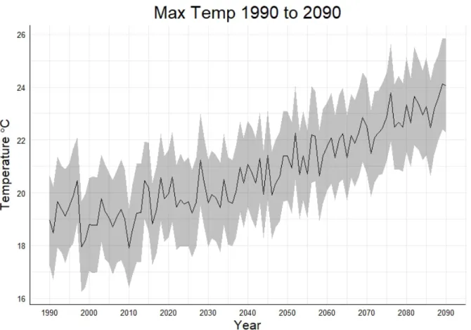
Epidemiological Disturbance Agent (EDA) extension. ... 33 Figure 10: Average maximum temperature of the 10 GCMs from 1990 to 2090 with

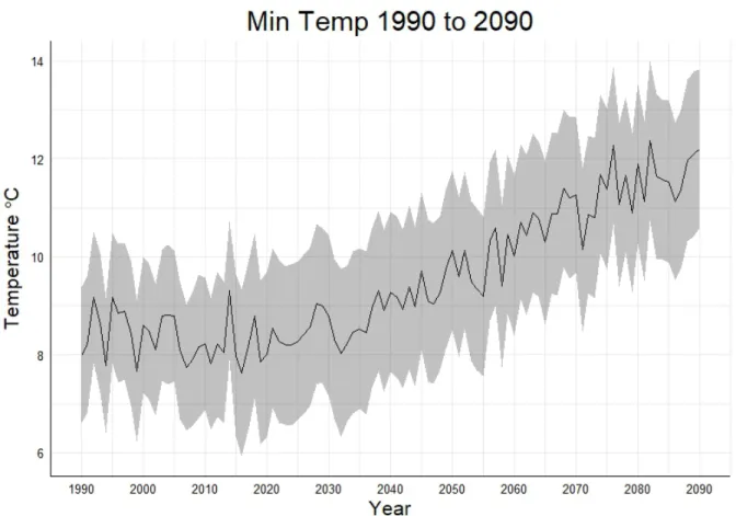
shaded grey region representing one standard deviation... 39 Figure 11: Average minimum temperature from the 10 GCMs from 1990 to 2090 in

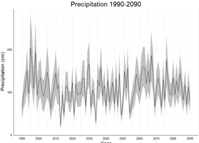
°C with shaded grey region representing one standard deviation. ... 40 Figure 12: Average annual precipitation from the 10 GCMs from 1990 to 2090 with

shaded grey region representing one standard deviation... 41 Figure 13: Aboveground carbon estimates for ecoregions in the Big Sur, CA from GNN

imputation and LANDIS-II at the beginning of the simulation (year 1990). ... 43

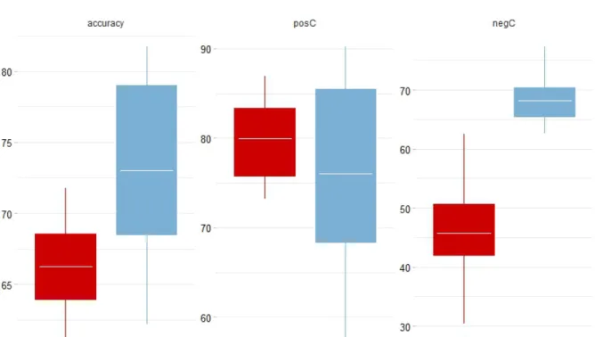
Figure 14: Boxplots of model accuracy comparison using the 2 methods full (all

comparisons at year 2013) and Yearly (model results compared to plot data for every sampling year). Accuracy = total model accuracy for both positive and negative disease status, posC = True positive identification (i.e. both plot and model results showed disease present), and negC = True negative

identification (i.e. both plot and model results showed no disease) ... 45 Figure 15: Ratio of Bay Laurel to Tanoak over time with shaded region representing

one standard deviation and the dark blue line representing the average from the 30 simulations ... 46 Figure 16: Average ratio of bay laurel to tanoak over time by ecoregion. Solid line

indicates the average and the shaded region represents the standard deviation. ... 47 Figure 17: Spatial modeling framework showing fire, disease, and forest composition.

These three components of the interactive landscape change over time and space, and interact with each other within and across time-steps. Sites also interact with each other within a time step. ... 51 Figure 18: Disturbance interaction theory and associated mechanism. Arrows

indicate direction of effect, top boxes are the disturbances, and bottom box is the response variable of interest, in this case forest composition. (a) and (b) are interaction chain which modify the likelihood of occurrence, while, (c) interaction modification modifies the magnitude or severity of the other disturbance. Figure modified from Foster et al. 2015. ... 52 Figure 19: Average # of fires, average fire size, average fire severity, and average #

of cohorts killed across the 30 simulations using the two disturbance scenarios with fire (fire, and fire and disease). Only fire severity is significant at a 0.05 confidence interval, p-value < 0.001. Both number of fires and average fire size show greater variability between simulations for fire and disease scenarios. ... 65 Figure 20: Average Fire Severity across ecoregions and entire landscape only

accounting for pixels within the fire perimeter. The p-values for each ecoregion

shown are significant at 95% confidence using a t-test with a Bonferroni p-value

adjustment: Mixed Evergreen = 0.0067, Redwood = 0.0071, Oak

Woodland = 0.0045, and the entire Big Sur = 0.0039, however, the other

ecoregions were not statistically significant compare across the 2

Figure 22: Ratio of bay laurel to tanoak over the course of the 100-year simulation for all 3 disturbance scenarios: fire, disease, and fire and disease. Solid line indicates the average and the shaded region is the standard deviation for the 30

simulations. ... 69 Figure 23: Ratio of bay laurel to tanoak over the course of the 100-year simulation

for 3 ecoregions for all 3 disturbance scenarios: fire, disease, and fire and disease. Solid line indicates the average and the shaded region is the standard deviation for the 30 simulations. ... 70 Figure 24: Ratio of bay laurel to coast live oak over the course of the 100-year

simulation for all 3 disturbance scenarios: fire, disease, and fire and disease.

Solid line indicates the average and the shaded region is the standard deviation for the 30 simulations. ... 71 Figure 25: Ratio of bay laurel to coast live oak over the course of the 100-year

simulation for 3 ecoregions for all 3 disturbance scenarios: fire, disease, and fire and disease. Solid line indicates the average and the shaded region is the standard deviation for the 30 simulations. ... 72 Figure 26: Ratio of bay laurel to California black oak over the course of the

100-year simulation for all 3 disturbance scenarios: fire, disease, and fire and disease. Solid line indicates the average and the shaded region is the standard deviation for the 30 simulations. ... 73 Figure 27: Ratio of bay laurel to California black oak over the course of the 100-year

simulation for 3 ecoregions for all 3 disturbance scenarios: fire, disease, and fire and disease. Solid line indicates the average and the shaded region is the standard deviation for the 30 simulations. ... 74 Figure 28: Bay Laurel over the course of the 100-year simulation for all 3

disturbance scenarios: fire, disease, and fire and disease. Solid line indicates the average and the shaded region is the standard deviation for the 30 simulations. ... 75 Figure 29: Tanoak over the course of the 100-year simulation for all 3 disturbance

scenarios: fire, disease, and fire and disease. Solid line indicates the average and the shaded region is the standard deviation for the 30 simulations. ... 76 Figure 30: Coast live oak over the course of the 100-year simulation for all 3

disturbance scenarios: fire, disease, and fire and disease. Solid line indicates the average and the shaded region is the standard deviation for the 30 simulations. ... 77

Figure 31: Bay Laurel over the course of the 100-year simulation for all 3

disturbance scenarios: fire, disease, and fire and disease. Solid line indicates

the average and the shaded region is the standard deviation for the 30 simulations. ... 78

Figure 32: Redwood over the course of the 100-year simulation for all 3

disturbance scenarios: fire, disease, and fire and disease. Solid line indicates

the average and the shaded region is the standard deviation for the 30 simulations. ... 79

Figure A1: Bay laurel to tanoak ratio over time movie. ... 103

Figure A2: Bay laurel to coast live oak ratio over time movie. ... 104

Figure A3: Bay laurel to California black oak ratio over time movie. ... 104

LIST OF ABBREVIATIONS

ANPP Above-ground Net Primary Productivity

C/N Carbon/Nitrogen

CA-BCM 2014 California Basin Characterization Model Downscaled Climate/Hydrology CAL FIRE California Department of Forestry and Fire Protection

CBH Base Height of the Crown

CO

Carbon Dioxide

CRM Component Ratio Method

CVS Current Vegetation Survey

DBH Diameter at Breast Height

EDA Epidemiological Disturbance Agent

FIA Forest Inventory Analysis

FLSM Forest Landscape Simulation Model

FMC Foliar Moisture Content

FWI Fire Weather Index

GCM Global Circulation Models

GDD Growing Degree Days

GNN Gradient Nearest Neighbor

ISI Initial Spread Index

LAI Leaf Area Index

LEMMA Landscape Ecology, Modeling, Mapping and Analysis NADP National Atmospheric Deposition Program

NECN Net Ecosystem Carbon and Nitrogen

NEE Net Ecosystem Exchange

NPP Net Primary Productivity

SHI Site Host Index

SHIMs Site Host Index Modifiers

SOD Sudden Oak Death

SOM Soil Organic Matter

SSURGO Soil Survey Geographic Database

CHAPTER 1: INTRODUCTION

Invasive Pest and Pathogen Problem

Invasive forest insects and pathogens are a significant threat to forested ecosystems worldwide (Liebhold et al. 1995; Vitousek et al. 1997; Simberloff 2000; Perles, Callahan, and Marshall 2010; Vitousek et al. 1996). As of 2010, a total of 455 non-native forest pests and 16 pathogens were discovered in the US; these organisms have become an increasingly serious threat to forest productivity and diversity (Aukema et al. 2010; Perles, Callahan, and Marshall 2010). Despite regulatory measures to prevent new introduction, the number of species has continued to increase annually (Aukema et al. 2011). Recently, awareness of both the economic and ecological impacts associated with introduced insects and pathogens has increased (Aukema et al. 2010).

For example, the emerald ash borer (Agrilus planipennis), Asian longhorned beetle (Anoplophora glabripennis), and sudden oak death (SOD) (Phytophthora ramorum) caused damages estimated to be in the billions of dollars due to lost timber resources (GAO 2006).

Another study estimated approximately $1.7 billion in local government expenditures and $830 million in lost property value from wood and phloem-boring non-native insects in the United States (Aukema et al. 2011). One study of emerald ash borer estimates that over the course of 10 years the cost to treat and remove infected ash trees would be $10.7 billion (Kovacs et al. 2010).

A study of oak wilt (Ceratocystis fagacearum) conducted in Anoka County, Minnesota found

that the cost of removal of dead trees would range from $18-60 million (Haight et al. 2011). In

the Big Sur region of California, the estimated cost of treatment was $7.5 million and property value loss was $135 million (Kovacs et al. 2011).

In addition to lost property value, these invasive forest pests and pathogens have serious consequences for ecosystem services and stability. These ecosystem effects include both short- and long-term effects. Short-term effects occur on timescales from weeks to years, while, long- term effects are seen over decades or centuries (Lovett et al. 2006). Direct short-term effects of forest and pathogen disturbance are tree defoliation, loss of vigor, or death. Indirect short-term effects of forest pests and pathogens include but are not limited to temporary decrease in primary productivity, increased exchange and leaching of nutrients, increased or decreased

decomposition, microclimate changes, and increased light availability (Lovett et al. 2006, 2004;

J. C. Jenkins, Aber, and Canham 1999). Long-term effects are primarily driven by a change in tree species competition due to host mortality differentiation, that leads to altered forest

structure, primary productivity, nutrient exchange rates, and soil organic matter production and turnover (Lovett et al. 2006). Three main attributes of the pest or pathogen affect the short- and long-term effects to ecosystem functions: mode of attack (how does a pest or pathogen attack the tree?), host specificity (generalist vs. specialist (one host vs. multiple hosts), Virulence (rapid mortality vs. slow mortality and probability of mortality) (Lovett et al. 2006). Additionally, there are important host tree characteristics that also play an important role in ecosystem

consequences: dominance (i.e. basal area or leaf area), succession and growth (pure stands vs.

The effects of forest pests and pathogens are typically long lasting due to 2 factors: host selectivity and persistence within the ecosystem (i.e. once established remain a permanent component of the ecosystem). For example, hemlock woolly adelgid has been shown to reduce forest floor moisture, increase rates of nitrogen accumulation, increase nitrate leaching into streams, decrease soil CO

efflux, and decrease stream flow in the summer (Den Boer 1968; J. C.

Jenkins, Aber, and Canham 1999; Ross et al. 2003; Yorks, Leopold, and Raynal 2003; Cobb, Orwig, and Currie 2006; Orwig et al. 2008). Cryphonectria parasitica, the causal agent of chestnut blight, has dramatically altered forest composition in the Eastern US; forests once dominated by American chestnut have become oak/hickory dominant. This is especially true in areas of the Appalachian Mountains where it is estimated that one in four hardwoods was an American chestnut (Jules et al. 2014; Prospero and Cleary 2017). The local dominance, biomass, or functional importance of species killed following infection or infestation determines the magnitude and nature of ecosystem change (Lovett et al. 2006; Ruess et al. 2009). Pathogen impacts range from dramatic stand level population declines to removals of single individuals and can occur over many years (Eviner and Likens 2008).

Modeling Pathogen Effects

Pest and pathogen models – frequently used to predict areas of future infection/infestation – have often ignored the effect of host heterogeneity and asymmetric host susceptibility and competency, except see (Meentemeyer et al. 2011; Fitzpatrick et al. 2012). Landscape epidemiological models frequently treat forest composition and host density as static (Meentemeyer, Haas, and Václavík 2012), meaning that the trees do not age or experience effects of disturbance. This makes it difficult to understand how disease alters species

composition at a landscape level (Cobb, Meentemeyer, and Rizzo 2010). Apparent competition

is a form of indirect competition driven by asymmetries in host susceptibility to a pathogen that lead to changes in species composition (Power and Mitchell 2004; Cobb, Meentemeyer, and Rizzo 2010). This lack of realistic changes in host community composition greatly impedes modeling the interactions of other landscape-level disturbances with disease spread (Cobb and Metz 2017). Combining a dynamic epidemiological model with a forest landscape simulation model (FLSM) allows for understanding how disease affects forest community composition and other disturbance dynamics and impacts.

Forest landscape simulation models (FLSMs) have been developed to specifically address management and research questions at landscape scales (>10

ha) by projecting forest dynamics over space and time (Mladenoff 2004; Scheller and Mladenoff 2007). These models typically include details such as tree age, species and biomass, and are widely used to analyze the influence of disturbances over time as they affect large-scale forest ecosystem dynamics (Thompson et al. 2016; Scheller and Mladenoff 2004). One of several FLSMs, LANDIS-II stands out as a process-based forest landscape model that can include variable time steps for different ecological processes (e.g. succession, disturbance, seed dispersal, forest management, carbon dynamics) and simulate their interactions as an emergent property of the independently simulated processed (Mladenoff 2005; Scheller and Mladenoff 2007; Mladenoff 2004).

LANDIS-II continues to grow its user community and several extensions are available to

simulate disturbances like wind, fire, insect spread, or land-use change. To date, the

Phytophthora Ramorum

Phytophthora ramorum is an oomycete, a fungus like eukaryotic microorganism, which

can infect over a hundred plant species (Rizzo, Garbelotto, and Hansen 2005; Davidson, Patterson, and Rizzo 2008). Disease symptoms are expressed in two forms: lethal infections on canker hosts and non-lethal foliar infections. The lethal form of the disease infects stems and branches of several ecologically important tree species, such as, tanoak (Notholithocarpus densiflorus), coast live oak (Quercus agrifolia), canyon live oak (Quercus chrysolepsis),

California black oak (Quercus kelloggii), and Shreve’s oak (Quercus parvula var. shrevei).

These canker hosts are epidemiological dead ends with the exception of tanoak (Kovacs et al.

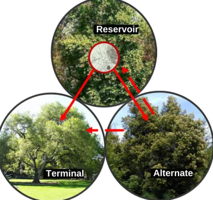
2011; Davidson et al. 2005). The foliar hosts can transmit the disease as leaves and twigs of these species produce inoculum. California Bay Laurel produces the most inoculum of all infected species and as such is consider the reservoir host with other hosts considered alternative hosts (Figure 1) (Kelly and Meentemeyer 2002; Meentemeyer, Rank, et al. 2008; Václavík et al.

2010). There are four main factors that make P. ramorum a serious threat to many forest

ecosystems: the potential for foliar hosts to readily support P. ramorum growth, the pathogen’s

ability to disperse by wind-blown rain (Davidson et al. 2005), the broad range of the host

species, and the ability to kill ecologically important species (Garbelotto, Rizzo, and Marais

2002; Rizzo and Garbelotto 2003).

Figure 1: Transmission pathways for the pathogen. Reservoir hosts = primary source of

pathogen spread indicated by the solid red lines, alternate hosts = able to spread pathogen but to a lesser extent indicated by the dashed red lines, and terminal hosts = no spread of the pathogen.

The range of sudden oak death is from the Big Sur region (Figure 3) of California to South-western Oregon (Meentemeyer, Rank, et al. 2008; Cobb, Meentemeyer, and Rizzo 2010;

Václavík et al. 2010; Cobb, Filipe, et al. 2012) (Figure 2). P. ramorum produces two types of spores: chlamydospores (resting spores) and zoospores, which have flagella for swimming.

Reservoir

Terminal Alternate

al. 2002). Transmission can be much higher than average during periods of high spring rain fall and much lower during periods of prolonged drought (Cobb and Metz 2017; Haas et al. 2016).

Figure 2: County level infection status of Sudden Oak Death as of 2016 (USDA Forest Service

Northern Research Station and Forest Health Protection 2016)

Economic costs of sudden oak death range from removal cost of dead trees, prevention cost, and loss of property value. One study estimated that over a ten year period the cost of treatment, removal, and replacement of 10,000 infected oaks was $7.5 million and that property losses to single family homes were $135 million (Kovacs et al. 2011).

Ecosystem consequences of SOD

P. ramorum is persistent within impacted stands, mortality is constant or increasing over

the scale of a decade, and inter-annual climate variability is critical to rates of pathogen spread (Davidson, Patterson, and Rizzo 2008; Cobb, Meentemeyer, and Rizzo 2010; Davis et al. 2010).

This dynamic interaction with its environment may prolong mortality and ecosystem effects of P.

ramorum over a greater time frame compared to other pests or pathogens especially those that

spread from discrete contact zones (Hansen and Goheen 2000; Rizzo, Slaughter, and Parmeter 2000; Kauffman and Jules 2006).

In plots affected by SOD, course woody debris accumulation rates increased in both snags and logs compared to uninfected plots (Cobb, Chan, et al. 2012). The number of large live tanoaks decreased dramatically in infected vs. uninfected plots, however, tanoak should be able to persist due to vegetative reproduction (i.e. seedlings or resprouting after fire) (Cobb, Filipe, et al. 2012). Additionally, in redwood-tanoak forests P. ramorum infection has led not only to a decline in large tanoak but also redwood while bay laurel became a more dominant part of the forests (Cobb, Meentemeyer, and Rizzo 2010). Thus, incorporating epidemiological processes, particularly factors that determine transmission and host biomass will yield more realistic

estimates of carbon accumulation over time and maximum amount of carbon released in infected

forests (Cobb, Chan, et al. 2012; Cobb and Metz 2017).

Fire Regime

The frequency of large wildfires in the western USA has increased significantly since the mid-1980s, together with warming temperatures and lengthened fire season (Beh et al. 2012).

Wildfire has played a crucial role in shaping the structure and ecological function of coniferous forests throughout the world, including those in the Big Sur area of California (Van Wagtendonk and Cayan 2008; Metz et al. 2010). The relationship between fire and fuels is that recently burned areas limit subsequent fire size by reducing fuel load. Thus, large areas of dense continuous fuels increase the likelihood that fires will become larger and more severe (Valachovic et al. 2011; He and Mladenoff 1999). Large, severe fires can lead to dramatic reductions in mature trees and aboveground and belowground live biomass, leading to cascading ecological effects (Cobb, Meentemeyer, and Rizzo 2016; Sturtevant et al. 2012).

Traditionally forest disturbance events that cause defoliation or damage to a stand are thought to increase fire severity and frequency due to an increase in litter accumulation and increased evapotranspiration due to greater light in the understory (McCullough, Werner, and Neumann 1998; Parker, Clancy, and Mathiasen 2006). However, recent empirical and modelling studies in pine bark beetle disturbance systems have shown that these disturbances are more interactive and may actually cause a decrease in fire severity. This is due to the nonlinear effects of increased dead fuel and thinned canopies (Romme et al. 2006; M. J. Jenkins et al. 2008;

Lynch and Moorcroft 2008). The long-term consequences of pathogen disturbance on fire

frequently considered a major agent of soil and land degradation, some have suggested that it is the single most important agent of geomorphological change (Neary, Ryan, and DeBano 2005).

Wildfire and pathogen/pest disturbances are key factors in hydrology of a region given that they have a large influence on evapotranspiration (Neary, Ryan, and DeBano 2005; Shakesby and Doerr 2006; Doerr et al. 2006).

Interacting Disturbances

Disturbances play an important role in maintaining or changing ecosystems. However, many disturbance regimes are being altered by climate change and other anthropogenic factors such as introduced species. Often times interacting disturbances have results that are unexpected based on the individual disturbances but when combined can lead to shifts from one ecosystem state to another (M. G. Turner 2010; Foster et al. 2015). Interactions between fire and disease can modify the other’s likelihood, intensity or spatial distribution.

Within the Big Sur study area of California there have been 2 years with large scale wildfires (2008 and 2016) since the establishment of the plot network in 2006. These fires have provided insights into how fire and SOD interact to affect forest composition and services. Forest floor carbon, nitrogen, and phosphorus were significantly greater in plots uninfected by P.

ramorum compared to those infected within the 2008 Chalk and Basin Complex fire burn area in

Big Sur. While no significant difference was found between infected and uninfected plots outside

of the burn area indicating that the interaction between fire and SOD have a meaningful impact

on post fire forest floor nutrient pools (Cobb and Metz 2017; Cobb, Meentemeyer, and Rizzo

2016).

Host fire tolerance and post fire recovery has feedbacks for disease prevalence, while selective host mortality by P. ramorum affects the standing and downed course woody debris which alters the fuel load of the forest thus affecting likelihood and severity of fires (Cobb, Meentemeyer, and Rizzo 2016; Metz et al. 2013, 2010). In some cases, wildfire could directly eliminate the pathogen from burned areas or at a minimum reduce the amount of disease and increase time until reinfection (Beh et al. 2012; Metz et al. 2010, 2013).

Goals

The goal of this dissertation is to use the LANDIS-II FLSM to examine how fire and

disease interact and how those interactions affect forest composition. There are two highly

important steps to be able to accomplish this goal. First, I needed to create an epidemiological

model that could interact with a forest composition model and fire model. Using this model at a

30-m spatial resolution to capture the spatial heterogeneity of the Big Sur was too slow to be

used for multiple simulation runs. Thus, I implemented the first parallelization in a FLSM to

improve computational time. I have divided the work into three chapters: (1) Parallelization in

FLSMs, (2) Dynamic Epidemiological Modelling in FLSMs: A Case Study Using P. ramorum in

Big Sur, CA, (3) Interacting Disturbances and Their Ecological Impacts: A Case Study Using

Fire and P. ramorum in Big Sur, CA.

CHAPTER 2: PARALLELIZATION OF FLSMS

Introduction

Forest landscape simulation models (FLSMs) are often used to understand and manage forest dynamics over space and time (Mladenoff 2004; Scheller and Mladenoff 2007). These models typically include details such as tree age, species, biomass and are widely used to analyze the influence of disturbances over time and space on forest ecosystem dynamics (Thompson et al. 2016). Among several types of FLSMs, LANDIS-II stands out as a spatially-explicit forest landscape model that can include variable time steps for different ecological processes (e.g.

succession, disturbance, seed dispersal, forest management, carbon dynamics) and simulate their

interactions (Mladenoff 2005; Scheller et al. 2007; Mladenoff 2004). LANDIS-II continues to

grow its user community and several extensions are made available to simulate disturbances like

wind, fire, insect spread, or forest pathogen spread and disease impacts. However, as the model

becomes more complex the computational time increases, requiring a tradeoff between spatial

extent and spatial resolution (Figure 4).

Figure 4: The tradeoff in computational time between resolution and extent. The log of both time and extent are shown here using a single-core model and number of computations for each combination of extent and resolution.

Parallel computing offers a means to reduce computational time by performing many

calculations simultaneously. This happens by dividing large calculations into smaller ones and

bringing the results back together when all calculations of one type are complete. Care must be

taken, however, to ensure that dependent processes still run sequentially. Parallelized FLSMs

linking of forest pathogen spread and tree mortality in forested landscapes. Thus, the feedback between pathogen spread and mortality can be predicted across space and time. The parallelized version of EDA is compatible with all succession extensions and can be used in conjunction with other disturbance extensions (e.g. fire, insect, wind) to simulate their combined effects on forest landscape dynamics. In this paper, we show that a parallel version of the model decreases

computational time proportional to the number of cores utilized for the model. This is done using an example application of the EDA extension in Big Sur, California.

Model description

The LANDIS-II modeling framework includes a model core that links, parses, and validates data from multiple extensions and allows the user to select a forest-succession extension and/or any number of disturbance extensions (Scheller et al. 2007). EDA is a disturbance extension compatible with all LANDIS-II forest-succession extensions. It is open source and freely available at the LANDIS-II project website: www.landis-ii.org. The download comes with an installer, user guide and sample data.

To date, no extension or core in LANDIS-II has taken advantage of the benefits of parallel computing. This is partially due to the core utilizing the Microsoft .Net Framework 3.5 instead of 4.0 or higher, which contain built in libraries for implementing parallel algorithms.

However, we exported the necessary libraries to a Dynamic-link library that allows us to utilize

the parallel functions within the .Net 3.5 framework.

Case study

To demonstrate the effect of parallelization, we ran the model for 20 years in an 8,017 km

area of central California at a 30-m resolution (total pixels = 885,588), USA with a 1-year time step. We averaged the time taken for a time step using 1, 2, 4, 6, and 8 cores on the same

computer; this is done in order to minimize differences in processor speeds. We then divided the total time for a time-step by the number of pixels in the study area in order to get a per pixel time-step. This allows us to scale up to multiple extents and resolutions as the main formula for computational time is number of pixels multiplied by time per pixel. The decrease in

computational time is directly related to the number of cores allocated to the model (1-8 in this

case), see Table 1. At some point when much higher cores are used on super computers this

relationship will break down and the decrease will no longer be 1:1 based on the amount of the

model that is parallel compatible. This extension is 100% parallelizable so Amdahl’s law

(McCool, Robison, and Reinders 2012) really takes effect at much larger core infrastructure

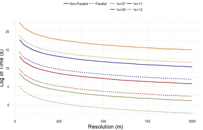
(around 64 cores). Figure 5 shows the difference in computational time at different resolutions

for a given extent. This means that the researcher can choose an extent 2 orders of magnitude

higher with the same resolution and have a similar computational time when using an 8-core

parallel model compared to the single core models that have been used previously.

Cores Time Speedup

1 29531 1

2 14621 2

4 7387 4

6 4907 6

8 3676 8

Table 1: Average time for a timestep for a simulation when allotted 1, 2, 4, 6, or 8 cores.

Figure 5: Relationship between the log of time and resolution with extent as factors. The parallel

model was ran using 8 cores on the same system as the single core.

Conclusion

We have shown that utilizing the parallel processing can significantly decrease the computational time. This allows the user to choose a spatial extent two orders of magnitude larger or a significantly smaller resolution at the same spatial extent without increasing the computational time. Turner et al (1989) determined that increasing spatial resolution results in the loss of low frequency landcover types (ecoregions) and species especially in areas with low clustering or high heterogeneity. The use of smaller resolutions can greatly increase the

understanding gained from processes occurring in highly heterogenous areas. Having shown that

parallelization can lead to dramatically lower computational time future work should continue to

utilize parallel computing and the opportunities it can provide.

CHAPTER 3: USING COUPLED DYNAMIC SPATIAL TEMPORAL

EPIDEMIOLOGICAL MODELS FOR UNDERSTANDING LONG-TERM FOREST COMPOSITION CHANGES WITH ASYMMETRIC DISEASE HOST-COMPETENCY

AND SUSCEPTIBILITY.

Introduction

Epidemiological disturbances, such as emerging pathogens and infectious disease outbreaks, are important agents of forest change around the world, causing tree mortality at scales ranging from individual trees of a single species to entire forest patches (Meentemeyer, Rank, et al. 2008; Welsh, Lewis, and Woods 2009). Beyond the complete loss of certain tree species, forest pathogens can significantly alter the functioning of forested ecosystems and the services they provide (Liebhold et al. 1995; Simberloff 2000; Vitousek et al. 1997). For example, pathogens can reduce the capacity of forests to sequester carbon, and can strongly interact with other types of disturbance such as fire, insects, and drought (Anderson et al. 2004; Dale et al.

2009; Elderd et al. 2013; Jactel et al. 2012; Vitousek et al. 1997). Coupled dynamic spatial temporal epidemiological models provide a predictive tool that can inform our understanding of how introduced forest pathogens alter forest ecosystem dynamics, which is crucial for land managers and decision makers (Cobb and Metz 2017; Rizzo, Garbelotto, and Hansen 2005).

One such emerging pathogen is Phytophthora ramorum, the causal agent of sudden oak death (SOD), which can infect over a hundred plant species (Rizzo, Garbelotto, and Hansen 2005; Davidson, Patterson, and Rizzo 2008). Disease symptoms are expressed in two forms:

lethal infections on canker hosts and non-lethal foliar infections. The lethal form of the disease

infects stems and branches of several ecologically important tree species, such as tanoak

(Notholithocarpus densiflorus), coast live oak (Quercus agrifolia), canyon live oak (Q.

chrysolepis), and California black oak (Q. kelloggii). These canker hosts are epidemiological

dead ends with the exception of tanoak (Kovacs et al. 2011; Davidson et al. 2005). The foliar hosts can transmit the disease as leaves and twigs of these species produce inoculum. California bay laurel (Umbellularia californica) produces the most inoculum of all infected species and as such is considered the reservoir host with other foliar hosts considered alternative hosts (Figure 1) (Kelly and Meentemeyer 2002; Meentemeyer, Rank, et al. 2008; Václavík et al. 2010).

One of the key effects that has surfaced at plot level analyses is the effect of apparent competition giving California bay laurel an advantage over tanoak (Cobb, Meentemeyer, and Rizzo 2010). Apparent competition occurs when 2 or more species share a common enemy (P.

ramorum) that has asymmetric effects on the host species (oaks, tanoak, and bay laurel). In

order to capture this effect over time, a ratio of bay laurel to tanoak was created, this ratio should increase if either or both of the following are true: (1) bay laurel increases faster than tanoak and/or (2) tanoak decreases while bay laurel increases or stays the same. Understanding how this emerging infectious disease will change forest composition requires the use of a dynamic

epidemiological model linked to a model that simulates forest growth and succession.

Forest landscape simulation models (FLSMs) have been developed to specifically address

management and research questions at landscape scales (>10

ha) by projecting forest dynamics

over space and time (Mladenoff 2004; Scheller and Mladenoff 2007). These models typically

different ecological processes (e.g. succession, disturbance, seed dispersal, forest management, carbon dynamics) and simulate their interactions as an emergent property of the independently simulated processes (Mladenoff 2005; Scheller and Mladenoff 2007; Mladenoff 2004).

LANDIS-II continues to grow its user community and several extensions are available to simulate disturbances like wind, fire, insect spread, or land-use change. To date, the

representation of forest pathogen and disease spread in FLSMs including LANDIS-II has been lacking.

Landscape epidemiological models frequently treat forest composition and host density as static (Cobb, Filipe, et al. 2012; Meentemeyer et al. 2011), meaning that the trees do not age or experience effects of disturbance. This makes it difficult to understand how disease alters competitive interactions among species, a process known as apparent competition, which can alter species composition at a landscape level (Cobb, Meentemeyer, and Rizzo 2010). Apparent competition can emerge when asymmetries in host susceptibility and tolerances to a pathogen drive changes in species composition (Power and Mitchell 2004; Cobb, Meentemeyer, and Rizzo 2010). Ignoring changes in host community composition limits the realism with which the interactions of other landscape-level disturbances with disease spread can be forecast through modeling (Cobb and Metz 2017).

Here I present the first case study of dynamic epidemiological modeling in a FLSM, utilizing LANDIS-II. The model couples the Net Ecosystem Carbon and Nitrogen (NECN) Succession extension to simulate forest succession and nutrient pools, with the new

Epidemiological Disturbance Agent extension (EDA) for LANDIS-II to simulate disease spread.

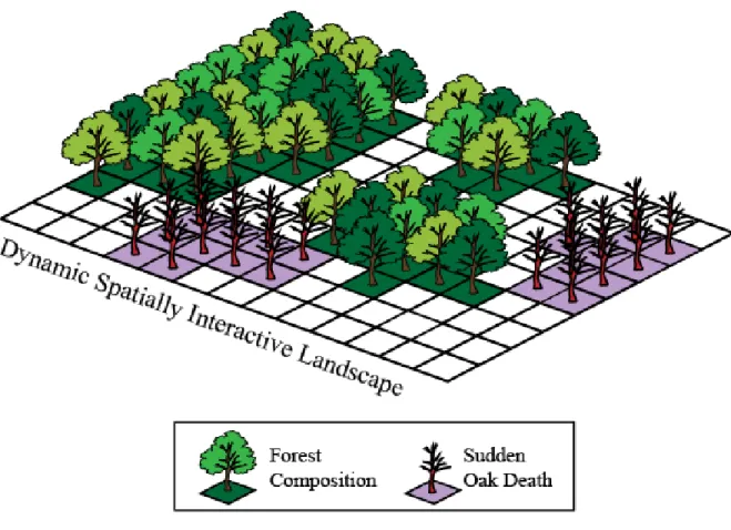
NECN will use a 10-year time-step and EDA will use a 1-year time-step (Figure 6). The model

will simulate P. ramorum spread and forest succession from 1990 to 2090 in Big Sur, CA using

projected daily climate data. The EDA model accounts for asymmetries in both host

susceptibility and competency and couples with the forest succession model to simulate forest composition changes across space and time. Utilizing models coupled in this way allows for examining changes in species composition due to apparent competition.

Figure 6: Spatial modeling framework showing disease and forest composition. These two

components of the interactive landscape change over time and space and interact with each

other within and across time-steps. Sites also interact with each other within a time step

in this area are frequently classified into two main categories, redwood and mixed evergreen.

There are many other ecosystem types in this study area and species composition varies even within these two broad classes. The topography in the study area is steep with deeply dissected slopes and drainages, elevation ranges from sea level to 1571 m within 5 km of the coast (Henson 1996). In 2006/2007 a long-term monitoring network for P. ramorum was established (Metz et al. 2010; Beh et al. 2012). The network consists of 280, 12.5 m radius plots throughout a 79,356 hectares study area within the Big Sur, CA. The plots were randomly located across a range of ecological conditions stratified by elevation, latitude, fire history, and forest community type (mixed evergreen and redwood forests). Plots were also located in areas with and without pathogen presence. All trees ≥1 cm in diameter at breast height (dbh) and shrubs that reached an area ≥ 1 m

were measured and species information recorded. P. Ramorum symptoms are

recorded for hosts that meet these requirements and tissue from symptomatic individuals is

brought to the lab for pathogen isolation (Davidson et al. 2005). All plots had plot centers

confirmed using survey-grade global positioning system receivers with a horizontal accuracy of

1 m or less after differential correction. A different subset of these plots were resampled in 2008,

2009, 2010, 2011, and 2013. These data will be used to supply LANDIS parameters and for

validation.

Modeling Framework

LANDIS-II is a process-based raster modeling framework consisting of a model core that links, parses, and validates data from multiple extensions (modules) and allows the user to “plug in” a forest succession extension and any number of optional disturbance extensions. Forests are represented as tree species-age cohorts (i.e. tanoak 100 for all tanoaks between 91-100 years) within raster cells across the landscape (Scheller et al. 2007). The NECN succession extension (version 4.1) and EDA extension (version 1.1) were utilized for this study.

Succession Extension

The NECN succession extension, originally developed as the Century Succession

extension (Scheller et al. 2011), is a combination of the original LANDIS biomass extension and the CENTURY Soil Organic Matter model (Parton et al. 1983). It simulates cohort growth, mortality, and regeneration based on life-history and physiological attributes. Species compete for resources within a grid cell and spatially disperse across cells within the landscape. This allows for species range shifts and the effects of apparent competition due to disease to play out.

Additionally, the model estimates above- and below-ground net primary production (NPP), net

ecosystem exchange (NEE), multiple pools of live and dead tree biomass (including leaf, wood,

fine root, course root, and course woody debris) and active, passive, and slow soil organic matter

pools (Parton et al. 1983; Scheller et al. 2011). NECN incorporates a climate library that allows

all extensions to utilize the same climate information. The climate data influences soil water

content and nitrogen available for tree growth. Growth and competition are simulated based on

limitation imposed by temperature, water, nitrogen, leaf area, and light availability instead of

operating at a photosynthetic level (Scheller et al. 2011).

Dynamic Epidemiological Extension

Base EDA requires a raster map with location(s) of initial infection. As well as agent- specific parameters such as host transmissivity, host susceptibility, climate tolerances and preferences, mean transmission rate, acquisition rate, maximum dispersal distance, and the appropriate dispersal kernel and exponent (see Sections 2.1-2.3 below). The model can also incorporate parameters defining how other disturbances modify likelihood of infection.

Base EDA is specifically designed to simulate asymmetric weather-driven transmission

of pathogen infection within a multi-host landscape. Transmission is modeled as a dynamic

process, affecting a meta-population comprised of N contiguous subpopulations represented by

cells (sites) arranged on a grid. Cells contain forest tree species age cohorts, and (optionally)

non-forest vegetation types. Tree mortality simulated by EDA is passed to the succession model

that in turn handles vegetation response to that mortality (e.g., changes in light, water, and/or

nutrients, depending on the succession extension used). Epidemiological disturbances within the

EDA are probabilistic at the site level, where each site is assigned a probability of being in one

of the following states: Susceptible (S), Infected (infectious non-symptomatic) (I), Diseased

(infectious and symptomatic) (D) (Figure 8).

Probabilities are compared with a uniform random number to determine whether the site

becomes infected or, if already infected, to become diseased. Disease causes species- and cohort- specific mortality in the cell. The epidemiological model is similar to that in Meentemeyer et al.

(2011) with adjustments made to fit the LANDIS-II framework and account for mortality.

Additionally, the model can handle more than one EDA agent (pathogen), especially those with aerial dispersal.

Site Host Index

Site host index (SHI) was adapted from the “site resource dominance” concept in the LANDIS-II Biological Disturbance Agent Extension (Sturtevant et al. 2004). SHI accounts for the spatial distribution of known hosts of the EDA agent and is a combined function of tree- species composition and the age cohorts present on that site. This approach allows the

quantification of susceptibility for each non-infected cell to become infected, and the suitability of each infected cell to produce infectious spores. The relative host index value of a given species cohort is defined by its host competency class, where low, medium, and high

competency classes are user-defined values ranging between 1 and 10, with non-hosts having a

value of 0. The EDA extension compares a look-up table with the species cohort list at each cell

generated by LANDIS-II to calculate SHI at time t using one of two methods: 1) the host value

from the maximum host competency class present, or 2) an average host value of all tree species

present, where the host value of each species is represented by the one assigned to the oldest

cohort. Species identified as “ignored” do not contribute to the calculation of average resource

value, while non-host species that are not ignored contribute a value of 0. Non-sporulating hosts

(i.e. hosts that do not contribute to pathogen or disease transmission) are not included in the host index calculation.

Site host index modifiers

Site host index modifiers (SHIMs) are optional parameters used to adjust SHI to reflect variation introduced by both site environment (i.e., landtype (ecoregion)) and recent disturbances (Sturtevant et al. 2004). Land type modifiers (LTMs) and disturbance modifiers (DMs) can range between -1 and +1, and are added to the SHI value of all affected sites where host species are present (SHI > 0). LTMs are assumed to be constant for the entire simulation, while DMs have a defined duration and decline linearly with the time since last disturbance ( 𝑡𝑡

) as follows:

𝐷𝐷𝐷𝐷

(𝑡𝑡) = 𝐷𝐷𝐷𝐷

∗

𝐷𝐷𝐷𝐷𝑑𝑑𝑑𝑑𝑑𝑑𝑑𝑑𝑑𝑑𝑑𝑑𝑑𝑑𝑑𝑑,𝐷𝐷𝐷𝐷𝐷𝐷

(Equation 1)

Disturbances that may affect a given EDA agent include fire, wind, other EDA agents and insects, as well as timber harvest. SHI is then modified by LTM and the sum of all DMs:

𝐷𝐷𝑆𝑆𝑆𝑆𝐷𝐷(𝑡𝑡) = 𝐷𝐷𝑆𝑆𝑆𝑆(𝑡𝑡) + 𝐿𝐿𝐷𝐷𝐷𝐷 + (𝐷𝐷𝐷𝐷

(𝑡𝑡) + 𝐷𝐷𝐷𝐷

(𝑡𝑡) + ⋯ ) (Equation 2) The user should calibrate the two modifiers to reflect the relative influence of species composition/age structure, the abiotic environment, and recent disturbance on SHI. SHIM is normalized by its mean over the entire study area, 𝐷𝐷𝑆𝑆𝑆𝑆𝐷𝐷(𝑡𝑡) =

𝐷𝐷𝑆𝑆𝑆𝑆𝐷𝐷_{𝑚𝑚𝑚𝑚𝑑𝑑𝑑𝑑}

, and modifies the

disease transmission rate, β (see Section 2.2). Normalization of SHI allows comparison of β to

Weather

An annual weather index, 𝑤𝑤(𝑡𝑡), is used to account for the effect of weather conditions on the probability of uninfected hosts becoming infected, and infected hosts sporulating and

spreading an individual EDA agent. Weather predictors (or transformations thereof) should be selected based on their relevance to the chosen EDA agent. The weather index is multiplied by a baseline transmission rate, 𝛽𝛽

, to produce a time-dependent transmission rate, 𝛽𝛽(𝑡𝑡) =

𝑤𝑤(𝑡𝑡)𝛽𝛽

, where 𝛽𝛽

is defined by the user. The basic weather index for year t, 𝑊𝑊(𝑡𝑡), comprises the cumulative effects of N weather predictors (e.g. rainfall alone, or rainfall and temperature) over a range of months, specified by the user (e.g. April to June), and is calculated as follows:

𝑊𝑊(𝑡𝑡) = ∑

𝑋𝑋

∗ 𝑋𝑋

∗ … ∗ 𝑋𝑋

(Equation 3)

where 𝑋𝑋

∗ 𝑋𝑋

∗ … ∗ 𝑋𝑋

represent the weather predictors and the cumulative-sum runs over days d included between two user-defined months ( 𝑚𝑚𝑚𝑚𝑚𝑚𝑡𝑡ℎ

and 𝑚𝑚𝑚𝑚𝑚𝑚𝑡𝑡ℎ

) for the current year t. If necessary, weather predictors in (1) can be replaced by derived (e.g., aggregated, or transformed) versions. As an example, a predictor can be aggregated (summed or averaged) over N

consecutive days of a week or month (e.g., cumulative precipitation). Transformed predictors are expressed by a function, ( 𝑋𝑋). In the current version of the extension (v1.0), only a polynomial transformation is available, defined as:

𝑓𝑓(𝑋𝑋) = 𝐴𝐴 + 𝐵𝐵 + 𝑒𝑒𝑒𝑒𝑒𝑒 (𝐶𝐶 ∗ �ln �

� 𝐸𝐸 ⁄ �

) (Equation 4)

where A, B, C, D, E, F are constants specified by the user to adjust the shape of the polynomial

(e.g., improving polynomial fit to empirical data on response of EDA agent to changes in

temperature). As an example, such a transformation can reflect changes in rate of pathogen

sporulation at increasing temperature values. The actual weather index, 𝑤𝑤(𝑡𝑡), is normalized by

the mean 𝑊𝑊

over the available time series of historical weather predictors: 𝑤𝑤(𝑡𝑡) =

𝑊𝑊(𝑡𝑡) 𝑊𝑊 ⁄

. Normalization means that 𝛽𝛽

can be interpreted as the annual transmission rate under average (or under constant) weather conditions. The weather index built this way varies annually, but is spatially uniform within each ecoregion.

Epidemiological Processes

The epidemiological model shares features with spatially-structured metapopulation models and relies on a few important assumptions: First, only the presence/absence of infection in each cell is accounted for. This simplification ignores a transient effect (occurrence, spread and intensification) within the same cell, assuming that an effective level of inoculum is reached rapidly (but still below the maximum sporulating capacity of the cell). Improving this

approximation would require a much larger computational effort in the parameter estimation procedure described in Filipe et al. (2012). Second, infected cells immediately become

infectious, which is particularly true for an EDA with a small latent period across its host range.

Third, infected sites remain infectious for an undetermined (i.e., long) period; hence no species can recover from infection throughout the simulation. However, if a cohort is killed by fire and resprouts, it is no longer infected.

At every time step t, a susceptible cell (site) i can become cryptically infected subject to a

force of infection Λ

(𝑡𝑡) and, once infected, it can become diseased at rate 𝑟𝑟

. Despite potentially

containing dead hosts, symptomatically infected (diseased) cells have the same transmission rate,

Δ𝑃𝑃_{𝑑𝑑,𝐼𝐼}

Δt

= Λ

(𝑡𝑡)𝑃𝑃

− 𝑟𝑟

𝑃𝑃

(Equation 6)

Δ𝑃𝑃_{𝑑𝑑,𝐷𝐷}

∆t

= r

𝑃𝑃

(Equation 7)

The initial conditions for each cell, at the estimated time of onset of the outbreak, are P

= 1, P

= 0, P

= 0, except at the cell estimated to be the location of the first infection, where P

= 0, P

= 1, P

= 0. The force of infection, Λ

(𝑡𝑡), is given by:

Λ

(𝑡𝑡) = 𝛽𝛽(𝑡𝑡) ∑ 𝐷𝐷𝑆𝑆𝑆𝑆𝐷𝐷

(𝑡𝑡) ∗ 𝐷𝐷𝑆𝑆𝑆𝑆𝐷𝐷

(𝑡𝑡) ∗ 𝑃𝑃

∗ 𝐾𝐾(𝑑𝑑

) (Equation 8)

where 𝛽𝛽(𝑡𝑡) = 𝑤𝑤(𝑡𝑡)𝛽𝛽

is the transmission rate, with 𝑤𝑤(𝑡𝑡) the annual index of weather fluctuation about a N-year average (see Section 2.2) and 𝛽𝛽

the baseline rate; 𝐾𝐾(𝑑𝑑

) is a dispersal kernel (see Section 2.3.1) for a given distance d between target and source cells; 𝑃𝑃

is the conditional probability that source cell j is infectious (either cryptic or symptomatic infection) given that target cell i is susceptible. To achieve a first order of approximation, we assume that 𝑃𝑃

≈ 𝑃𝑃

+ 𝑃𝑃

which we expect to be a reasonable approximation to the infection pattern, especially when dispersal is not too localized (e.g. within short distance from source of infection).

Dispersal kernel

The dispersal kernel used in Base EDA is derived from, and shares code with, the seed

dispersal kernel developed by Lichti and colleagues (N. Lichti, Purdue University, unpublished

manuscript). This dispersal function and associated distributions are especially suitable for

aerially dispersed EDA agents including a range of fungi, bacteria, and mistletoes. The

probability that the agent disperses a distance d from the source was expressed by two main

functional forms, often used in the literature: a power-law and a negative exponential. Their

generic form can be defined as follows:

𝐾𝐾

(𝑑𝑑) = 𝑑𝑑

(Equation 9) 𝐾𝐾

(𝑑𝑑) = 𝑒𝑒

(Equation 10)

An EDA agent produced in a source cell can only be deposited in a cell different from the source, i.e., transmission in force of infection ( Λ, see Section 2.3 above) is conditional on the agent being dispersed outside the source cell. The rationale for this choice is that infection processes within a cell are not tracked (no transient effect). In addition, the kernel must integrate to 1 within a chosen 2D spatial neighborhood window (excluding the source cell). The 2D window accounts for all possible pathways through which the target cell can become infected by a given source cell. A user-defined maximum radial distance is used to limit EDA agent dispersal within a chosen neighborhood size. For cases where only local, short-distance dispersal events are considered, this parameter becomes essential to reduce computational burden. Only isotropic dispersal (no wind-assisted directional spread) was considered for version 1.0 of the Base EDA extension.

Tree species cohort mortality

Within each diseased cell, the mortality of individual tree species age cohorts is a

probabilistic function of the mortality probability of the cohort’s vulnerability class. The user

defines which species and ages fall into each vulnerability class (low-high), and the probability

of cohort mortality for each class. Probabilities are compared with a uniform random number to

level processes or dynamics it should not cause significant changes in outcome. The Base EDA time step concludes updating the time since last disturbance, outputting maps of cell states (1 = Susceptible, 2 = Infected, 3 = Diseased) and cohort mortality, and by updating the Base EDA log file (Figure 9).

Figure 9: Flow diagram illustrating the main logical structure of the LANDIS-II Base Epidemiological Disturbance Agent (EDA) extension.

Model Inputs

LANDIS-II model inputs include initial vegetation data, ecoregion data, species and

functional group trait data, epidemiological data, and climate data (Table 2). See Appendix 1 for

all tables with NECN and EDA extension parameters.

Table 2: Data and Sources.

Parameter Groups Source Data

Species Specific

Silvics Manual, Literature, LEMMA GNN

Seed dispersal; fire regeneration; resprout probability; resprout age limits; shade, fire, and drought tolerance; sexual maturity;

longevity; min temp; GDD min and max;

leaf, wood, and root lignin and C/N ratios.

Functional Groups

Silvics Manual and previous Century models

Mortality shape curves; max LAI; growth parameters; leaf drop month; and fraction of carbon in fine and course roots.

Ecoregion Types LandFire Biophysical Regions

Groups regions with similar climate, topography, and soil

Ecoregion Parameters SSURGO, NADP Soil depth; percent clay; percent sand; field capacity; wilting point; drainage; nitrogen Climate (Daily) CA-BCM 2014 Precipitation, TMIN, TMAX, Wind

Acronyms: LEMMA = Landscape Ecology, Modeling, Mapping & Analysis, GNN = Gradient Nearest Neighbor, GDD = growing degree days, C/N = Carbon/Nitrogen, LAI = Leaf Area Index, SSURGO = Soil Survey Geographic Database, NADP = National Atmospheric Deposition Program, CA-BCM 2014 = California Basin Characterization Model Downscaled Climate and Hydrology.

Vegetation Data

Initialization of the current vegetation on the simulated landscape, used the gradient

nearest neighbor (GNN) map for the California Southern Coastal Range (map region 233)

produced by the Landscape Ecology, Modeling, Mapping and Analysis (LEMMA) group for the

Northwest Forest Plan Effectiveness Monitoring (Ohmann et al. 2011; Ohmann and Gregory