Skilled Unskilled Wage Asymmetries as an Outcome of Skewed International Trade Patterns in the South

Munich Personal RePEc Archive

Skilled-Unskilled Wage Asymmetries as

an Outcome of Skewed International

Trade Patterns in the South

Mamoon, Dawood

University of Islamabad

6 November 2017

Online at

https://mpra.ub.uni-muenchen.de/82449/

Skilled-Unskilled Wage Asymmetries as an Outcome of Skewed International Trade Patterns in the South

DAWOOD MAMOON*

Dean and Professor

School of Economics and Management University of Islamabad

(Harvard University Affiliate: 2013-2017) (George Mason University Affiliate: 2016-2018) (Member World Economic Survey Expert Group)

(November, 2017)

Abstract

The paper tries to find out the impact of trade liberalization on income inequality. The literature suggests that trade favors one segment of the society over other and cause uneven development. For example, one possible way through which inequality is suspected to seep into the economy through processes of liberalization is by increasing the relative wages of skilled labor as compared to the unskilled ones. Empirical evidence is provided to this effect by employing Theil Wage inequality Index and up to 28 different concepts of openness/ trade policy. OLS as well as 2SLS regressions with numerous specifications were run. It is found out that openness not only causes wage inequality but the relationship is significant for the developing countries. Additionally, the study also suggests that human capital, which is accrued from liberalization processes, is responsible for amplifying wage inequality.

“Openness and trade liberalization are now seen almost universally as key components of the national policy cocktail required for economic growth and aggregate economic well being. They are believed to have been central to the remarkable growth of industrial countries since the mid- 20th _{century and to} the examples of successful economic development since around 1970. The continued existence of widespread and abject poverty, on the other hand, represents perhaps the greatest failure of the contemporary global economy and the greatest challenge it faces as we enter the 21st

century.”………..Alan Winters (2000).

“Comprehensive trade reform can be helpful in reducing poverty provided it is accompanied by appropriate enabling policies.”………..Global Poverty report (World Bank, 2001a)

1. Introduction:

Many studies have tried to capture the relationship between trade liberalization and

income inequality. A recent paper by the two well known World Bank economists,

Dollar and Kraay (2004), concludes that liberalization does not carry any significant

effects on income distribution and at best the relationship is of neutral nature.

However their results have been challenged by many on the basis of their

methodology and variable choice (i.e., see Ravallion, 2003; Amann et al, 2002;

* _{The author is grateful to Mansoob Murshed (ISS) for his comments and Andrew K Rose (UCL,}

Srinivasam and Bhagwati, 2002). Murshed (2003) pointed out that Dollar and Kraay

only considered successful globalizers, mainly from Asia, in their analysis and

excluded the unsuccessful globalizers from their sample in order to capture trade

and poverty relationships.

Furthermore there is ample empirical evidence in the literature which rejects the

notion that trade is insignificantly related with inequality. For example, Behrman et

al (2001) noticed that in 7 out of 18 Latin American countries that initiated market

reforms in the mid 1980s, inequality has actually increased in recent times. The rest

of the economies in their sample showed that inequality was approximately same in

1990s to the levels of 1980s. Jayasuriya (2002), though accepted that liberalization

has reduced consumption poverty in South Asia, showed skepticism concerning

neutral distributional effects of liberalization. A more clear line is adopted by single

country case studies. Many suggest that the distribution of the positive effects of

liberalization is some what skewed towards urban households rather than rural and

wealthy households rather than poor.1 _{It is further noticed in many studies}2 _that

liberalization process in many developing countries seems to be biased against

low-skilled labor. The empirical verification in this regard comes mainly from Latin

American region primarily because most of the economies in the region undertook

rigorous reform policies in the mid 1980s as part of their structural adjustment plans

and also witnessed grappling inequality in Post reform periods. Ligovini et al (2001)

found out that inequality in Mexico rose sharply between 1984 and 1994 and rising

returns to skill labor accounted for 20 percent of the increase in the inequality in

household per capita income. Similarly, Hanson and Harrison (1999) found that the

reduction in tariffs and the elimination in import licenses account for 23 percent

increase in the relative wages of skilled labor over the period of 1986-1990 thus

providing evidence for the role liberalization played in rising inequality in Mexico.

Other country studies on Brazil, Chile, Colombia and Venezuela, also show that

skilled workers received increased premiums after liberalization when compared to

their unskilled counterparts (World Bank, 2001b).Such empirical evidence

1 _{See for example, Chen and Ravallion (2003), Cockburn (2001), Friedman(2000), Lofgren (1999).}

contradicts the basic trade theory which suggests that trade liberalization would

result in an increase in demand for low-skilled in a developing country, thereby

improving the relative earnings of this group compared with the more skilled. The

evidence further feeds the fears of Ravallion (2003) that openness to trade can lead

to the demand for relatively skilled labor, which tends to be more inequitably

distributed in poor countries than rich ones. He also proposed caution regarding the

results of David and Dollar (2004) paper concerning neutral inequality effects of

trade reform on the base of latter’s methodology and referred to his own empirical

work which found that reform process do carry unequal distributional effects.

2. Trade Liberalisation and Movements in Relative Wages:

We employ the UTIP-UNIDO wage inequality ‘THEIL’ measure calculated by

University of Texas Inequality Project (UTIP), instead of taking measures of absolute

inequality which captures the personal income distribution i.e. GINI. This is because

we are more interested in the functional distribution of income. Changes in the

functional distribution between skilled and unskilled labour, will in turn predictably

impact on the personal income distribution in countries that are unskilled labour

abundant. Inequality will rise as the skilled-unskilled labour wage premium increases

and vice versa. Since, the Theil Index is based on UNIDO 2001, the wages of skilled

and unskilled labor represent sectoral wage rates, including manufacturing industries

for which the UNIDO Industrial Statistics Database (UISDB) provides detailed

time-series data for most countries in the world.

The basic formula of Theil index is as follows.

………..(1)











          

 

   

 

 n

i

i n

j j i

x x

x x Theil

1

mean torelative income

incomeaggregate of

share is weight

1

ln



Whereas under perfect equality, i.e. everybody gets the mean income, the index

takes the value equal to zero:

……….(2)

 







However in the case of perfect inequality, one person takes all and everyone else

gets nothing. The individuals can be ordered in the sum from i=1,...,n from lowest to

highest income.

……..(3)

 

0 

                                                   





The value of Theil index depends upon the size of the population, as in (3). For

example, consider a society with two people where one person has everything and

compare it to a society with four people where one person has everything, also.

Which society is more unequal? There are more poor persons per rich person in the

society of four people, so the Theil index will be greater in that case. The UTIP

dataset provides the Theil index for nearly 160 developing and developed countries,

and the time series spans 40 years, from the early 1960s to the late 1990s.

Figure 1 illustrates trends in wage inequality over time in selected developing

countries and is representative of different regions. All the country graphs, except

one, show that wage inequality has been on the rise in 1980s and 1990s. The only

exception is Singapore which belongs to group associated with the “East Asian

Miracle” of the 1980s. This miracle, however, is confined to a few countries, and is

not representative of the developing world, as is evident from above graphs. Since

5 In d ia 0 0 .0 2 0 .0 4 0 .0 6 0 .0

8 0.1

0 .1 2 19 63 19₆₅ 19₆₇ 19 69 19 71 19₇₃ 19₇₅ 19 77 19 79 19 81 19₈₃ 19₈₅ 19 87 19 89 19₉₁ 19₉₃ 19 95 19 97 19 99 Y e a rs Wage Inequality P a k is ta n 0 0 .0 1 0 .0 2 0 .0 3 0 .0 4 0 .0 5 0 .0 6 0 .0 7 0 .0 8 19₆₃ 19 65 19 67 19 69 19₇₁ 19 73 19 75 19 77 19₇₉ 19₈₁ 19 83 19 85 19 87 19₈₉ 19 91 Y e a rs Wage Inequality Z im b a b w e 0 0 .0 1 0 .0 2 0 .0 3 0 .0 4 0 .0 5 0 .0 6 0 .0 7 0 .0 8 0 .0 9 19 63 19 65 19 67 19₆₉ 19 71 19 73 19 75 19 77 19₇₉ 19₈₁ 19 83 19 85 19₈₇ 19₈₉ 19₉₁ 19 93 19 95 19₉₇ Y e a r Wage Inequality B a n g la d e s h 0 0 .0 1 0 .0 2 0 .0 3 0 .0 4 0 .0 5 0 .0 6 0 .0 7 0 .0 8 0 .0 9 19₆₇ 19 69 19 71 19 73 19 75 19₇₇ 19 79 19₈₁ 19 83 19₈₅ 19₈₇ 19 89 19₉₁ Y e a rs Wage Inequality S in g a p o re 0 0 .0 2 0 .0 4 0 .0 6 0 .0

8 0.1

0 .1 2 0 .1 4 1963 1965 1967 1969 1971 1973 1975 1977 1979 1981 1983 1985 1987 1989 1991 1993 1995 1997 1999 Y e a rs Wage Inequality Ja m a ica

0 0.05 0.1 0.15 0.2 0.25 0.3 0.35

19 63 19₆₅ 19 67 19₆₉ 19 71 19₇₃ 19 75 19 77 19₇₉ 19 81 19₈₃ 19 85 19 87 19₈₉ 19 91 Y e ar Wage Inequality C h in a 0 0 .0 0 0 5 0 .0 0 1 0 .0 0 15 0 .0 0 2 0 .0 0 2 5 0 .0 0 3 0 .0 0 3 5 0 .0 0 4 0 .0 0 4 5 19 7 7 19 7 8 19 7 9 19 8 0 19 8 1 19 8 2 19 8 3 19 8 4 19 8 5 19 8 6 Y e a rs

Wage Inequality many deve

lopi ng cou ntries e mb raced l ib e rali zatio n, it is

safe to imp

ly that th

e ab ove tre n ds i n wage inequ ali ty is re late d

to these m

arke t reform s. Figu re 1: C o lo m b ia 0 0 .0 1 0 .0 2 0 .0 3 0 .0 4 0 .0 5 0 .0 6 19 63 19 65 19₆₇ 19₆₉ 19 71 19₇₃ 19₇₅ 19 77 19 79 19₈₁ 19₈₃ 19₈₅ 19 87 19 89 19₉₁ 19 93 19 95 19₉₇ 19₉₉ Y e a rs Wage Inequality C h ile 0 0 .0 2 0 .0 4 0 .0 6 0 .0

8 0.1 0.12

The object of this paper is to see whether this proposition holds across some 124

developing countries and economies in transition. Appendix 3 lists these countries,

and the latest year for which the Theil wage inequality index was available for them.

To this effect the paper initially proposes a simple OLS regression model:

………..(4) i

i i

i

i OPEN HK Disteq

THEIL     

Where THEIL_i is wage inequality in country i, OPEN_iand HK_iare respectively

measures for openness/trade policy and human capital and _i is the random error

term, whereasDisteq_i (distance from the equator) is a proxy for geography.

Inclusion of human capital and geography variables will enhance the explanatory

power of our model because on the one hand human capital plays important role in

inequality in a post liberalization period since international trade favors skilled labor

over unskilled and on the other hand country locations determine patterns of trade

subsequently affecting inequality.

Figure 2

Openness (Exports+Imports/GDP, 1985) , Tariffs (Import Duties as a % Imports, 1985) and Wage Inequality (Theil Index, 1997)

Before undertaking any regression analysis, let us take a look at simple graphs (figure

2) showing bi-variate relationship between openness and inequality. The first graph

in the figure shows that trade shares are positively related with increases in

Afghanistan

Angola United Arab Emirates

Argentina Azerbaijan Burundi Benin Burkina Faso Bangladesh Bulgaria Bahrain Bolivia Brazil Bhutan Botswana Central African Republic Chile

China Cote d'Ivoire

Cameroon Congo, Rep. _{Cape Verde}

Costa Rica Cyprus Dominican Republic AlgeriaEcuador

Egypt, Arab Rep. Eritrea

Ethiopia Fiji Gabon

Georgia Equatorial Guinea

Hong Kong, China

Honduras Croatia HaitiIndia

Iraq Jamaica Jordan Kenya Korea, Rep. Sri Lanka Lesotho Lithuania Latvia Macao, China Moldova Myanmar Mozambique Mauritius Malawi Nigeria Nicaragua Nepal OmanPanamaPeru Pakistan

Papua New GuineaRomania Rwanda

Saudi Arabia Sudan

Senegal SurinameSlovak Republic Slovenia Swaziland Seychelles Togo

Tonga Trinidad and Tobago Tunisia Turkey Tanzania Uganda Ukraine Uruguay Uzbekistan St. Vincent and the Grenadines

Samoa Yugoslavia, Fed. Rep.Zambia

0 .2 .4 .6 .8 W a g e I n e q u a li ty

2 3 4 5 6

Openness

Theil97 Fitted values

Afghanistan

United Arab Emirates Azerbaijan Burundi Burkina FasoBenin

Bulgaria

Bahrain Bolivia Brazil

Botswana Central African Republic_Chile

Cote d'Ivoire Cameroon Congo, Rep. Cape Verde Dominican Republic Algeria Ecuador Eritrea Ethiopia Fiji Gabon Georgia Equatorial Guinea Croatia India Jamaica Jordan Korea, Rep. Lithuania Macao, China Moldova Mauritius MalawiNigeria Nicaragua Nepal Oman Panama Peru Rwanda Saudi Arabia Sudan SenegalSlovenia Seychelles Togo Tonga Trinidad and Tobago Tunisia Turkey Tanzania Ukraine Uruguay Uzbekistan

St. Vincent and the Grenadines Samoa Zambia 0 .2 .4 .6 .8 W a g e I n e q u a li ty

0 .5 1 1.5

trade policy(tariff rates)

inequality and confirms our hypothesis that international trade is biased towards the

wages of skilled labor in developing countries. However interestingly, the second

graph in figure 2 fails to develop any definite association between tariffs3 _and

inequality substantiates the findings of Dollar and Kraay (2004) that the relationship

between integration and inequality is at best insignificant. Well the lesson which can

be drawn from figure 2 is that the choice of openness/trade policy variable matters

apropos its relation with inequality. This calls for a robustness check.

To this effect the OLS regression analysis (Appendix 1) utilizes several concepts of

openness and trade policy in addition to trade shares and tariff rates. Here a study

by Rose (2004) has been of great use because his paper identifies nearly 60 different

measures of openness/trade policy. 28 of these measures, which suit the data

requirements, are employed in this paper (Please refer to Appendix 2 which gives

detailed information about these measures). Nevertheless our core openness

variable remains to be overall trade share (the ratio of nominal imports plus exports

to GDP).

As far as the signs of the coefficients of 28 openness/trade policy variables are

concerned, Tables 1a and 1b show that they have been overwhelmingly positive

under all specifications satisfying the assertion that openness is positively associated

with increased wage inequality. However the coefficients have very small values

suggesting limited role they play in explaining inequality. Small 2values with any of

R

the specifications of Eq (4) suggest the same. Additionally only 7 out of 28

openess/trade policy concepts have turned out to be significant which suggest that

the relationship between trade and inequality is weak in nature. In the light of these

results we cannot confidently claim that openness cause increased relative wage

inequality by favoring skilled labor.

The OLS regression though useful is always suspected to suffer from econometric

problems such as endogeneity among variables especially under cross section

analysis. Though Geography is a pure exogenous variable here, the level of

integration of an economy depends upon its location in the world map (Rodrik et al,

2004). Similarly, human capital depends on the fact how open a country is. Though

simple Stolper-Samuelson theory would suggest that the returns to skill would

decline and with them incentives for education when a skilled-scarce developing

country opens up (see Wood and Ridao-Cano, 1999), in a multidimensional Stolper

Simuelson model which is nearer to real life, endogenous growth with constant

returns to R & D or skills-bias in tradables as oppose to non tradables could very well

lead to increase in returns to education upon openness (Arbache et al, 2004).

Openness can also lead to more efficient education technologies thus improving the

level of human capital in a country (Winters, 2004). Here we have to extract the

dependency of trade policy/openness on human capital by finding a right instrument

for the former variable.

The literature clearly establishes that predicted trade shares following Frankel and

Romer (FR) (1999) from the gravity equation is the most appropriate instrument for

openness/ trade policy ( see, Dollar and Kraay, 2002; Rodrik et al, 2004; Acemolgu,

Johnson and Robinson, 2001; Hall and Jones, 1999). Furthermore, following the likes

of Rodrik et al (2004), distance from the equator has been chosen as the second

instrument for openness/trade policy variables.

Our Instrumental Variable (IV) Regression (or 2 Stage Least Square) model has two

equations

………(5) i

i i

i OPEN HK

THEIL    ₁

………(6) i

i i

i FR Disteq

OPEN    ₂

Here FR_i stands for predicted trade shares from gravity equations computed by

United Arab Emirates Burundi Burkina Faso Bulgaria Bolivia Brazil Bhutan Botswana

Central African Republic Chile

Cote d'IvoireCameroon

Congo, Rep. Cape Verde Dominican Republic Algeria Ecuador EritreaEthiopiaFiji Gabon Georgia Equatorial Guinea

Hong Kong, China Croatia

HaitiIndia Iran, Islamic Rep.

Iraq Jamaica Jordan Korea, Rep. Sri Lanka Macedonia, FYR Mauritius Malawi Nigeria Nicaragua Nepal Oman Pakistan

PanamaPeruPapua New Guinea Saudi Arabia Sudan Senegal Slovenia Seychelles Togo Tonga Trinidad and Tobago

Tunisia Turkey Tanzania

Ukraine

Uruguay

St. Vincent and the Grenadines Yugoslavia, Fed. Rep.

South Africa Zambia 0 .0 5 .1 .1 5 W a g e I n e q u a li ty

2 3 4 5 6

Openness(predicted)

Fitted values Fitted values

United Arab Emirates Burundi Burkina Faso Bulgaria Bolivia Brazil BhutanBotswana

Central African Republic Chile Cote d'Ivoire Cameroon Congo, Rep. Cape Verde Dominican Republic AlgeriaEcuador Eritrea EthiopiaFiji Gabon Georgia Equatorial Guinea Hong Kong, ChinaCroatia

Haiti India

Iran, Islamic Rep. Iraq Jamaica Jordan Korea, Rep. Sri Lanka Macedonia, FYR Mauritius Malawi Nigeria Nicaragua Nepal Oman Pakistan Panama Peru Papua New Guinea

Saudi Arabia Sudan Senegal Slovenia Seychelles Togo Tonga

Trinidad and Tobago

Tunisia Turkey

Tanzania Ukraine

Uruguay St. Vincent and the Grenadines

Yugoslavia, Fed. Rep. South Africa Zambia 0 .0 5 .1 .1 5 W a g e I n e q u a li ty

-.1 0 .1 .2 .3 .4

trade policy(predicted tariff rates)

Fitted values Fitted values

In the 1st _{stage, equation (6) has been used to generate predicted values of}

openness/ trade policy variables by regressing them on the two instruments. The

predicted openness/trade policy variables are then employed in equation (5) as the

second and final stage of IV regression analysis. Please note that the only difference

between eq (5) and equation (4) is that the former does not carry Disteq_i variable

which is instead used as an instrument in eq (6).

Before we carry out the IV analysis, let us look at simple bivariate graphs between

predicted trade shares and predicted tariff rates with Theil index to see whether this

time we can get a clearer picture regarding openness inequality relationship. Figure

3 visibly shows that inequality moves positively with openness. The predicted values

of openness/trade policy provide a much clear trends in openness-inequality

movements. On the one hand the first graph of figure 3 shows that increase in trade

shares after liberalization leads to higher inequality and on the other hand the

second graph suggests that decrease in tariffs carries unequal distributional effects

on wages. One of the reasons for decrease in relative wages of unskilled labor, as

tariffs fall, is that the heavily protected sectors in many developing countries tend to

be the sectors that employ a high proportion of unskilled workers (Goldberg and

Pavcnik, 2004).

Figure 3

Table 2 (Appendix 1) gives IV regression results with 58 different specifications. The

results confirm the findings of figure 3. All openness/ trade policy variables carry

expected signs and nearly all of them are significantly related with wage inequality.

Under the light of these results it can be safely suggested that trade liberalization

significantly worsens the distribution of wages among skilled and unskilled labor in

developing countries. Further more, human capital is negatively related to inequality

showing that the countries which start out with relatively developed human capital

do well apropos wage inequality. This is an expected result and in line with theory

that the countries, where human capital is evenly distributed, are less prone to

adverse wage distributions among labor (Fisher, 2001; Tuelings and Van Rens, 2002;

Eiche, 2001; and Bourguignon and Morrisson, 1990; Tilak, 1989).

3. Human Capital, Trade and Unequal Wages:

According to Tinbergen (1975) inequality is determined by the opposing effects that

technology (skilled labor demand) and education (skilled labor supply) exerted on

the relative wages. Following the line proposed by Tinbergen, the role of human

capital vis-à-vis inequality becomes complex once we bring trade liberalization into

the picture as trade effects the demand of skilled labor through technology transfer

and processes of learning by doing. For example, human capital under liberalization

can cause wage inequality in a developing country, where there is unequal

distribution of skilled and unskilled labor, because global integration cause upward

pressure on the wages of the skilled labor as demand of skilled labor exceeds its

supply

Recently, Eiche et al (2001: 19) accepted this fact and suggested that human capital

plays a dual role in development because the stock of educated workers in an

economy determine both the degree of income inequality and the rate of growth,

and the parameters of the demand for and supply of labor are crucial determinants

of whether inequality increases or decreases as an economy accumulates human

Afghanistan

Angola

Albania

United Arab Emirates Argentina Burundi Benin Burkina Faso Bangladesh Bulgaria Bahrain Bahamas, The_Belize

Bolivia Brazil

Barbados Bhutan Botswana

Central African Republic Chile China Cote d'Ivoire Cameroon Congo, Rep. Colombia Cape Verde Costa Rica Cuba Cyprus Dominican Republic Algeria Ecuador Egypt, Arab Rep.

Ethiopia Fiji Gabon Ghana Guinea Gambia, The Equatorial Guinea Guatemala

Hong Kong, China Honduras Haiti

Indonesia India

Iran, Islamic Rep.Iraq

Jamaica Jordan

Kenya Korea, Rep. Kuwait

Liberia Libya Sri Lanka Lesotho Morocco Madagascar Mexico Myanmar Mongolia MozambiqueMauritania Mauritius Malawi Malaysia Namibia Nigeria Nicaragua Nepal Oman Pakistan Panama Peru Philippines Papua New Guinea

Puerto Rico Paraguay Qatar Romania Rwanda Saudi Arabia Sudan Senegal Singapore El Salvador Somalia Suriname Swaziland Seychelles Syrian Arab Republic

Togo Thailand

Tonga

Trinidad and Tobago Tunisia

Turkey

Tanzania Uganda

Uruguay

St. Vincent and the Grenadines

Venezuela, RB Samoa Yemen, Rep.

Yugoslavia, Fed. Rep.

South Africa Zambia Zimbabwe 4 5 6 7 8 H u m a n C a p ita l

2 3 4 5 6

trade policy(predicted openness)

Fitted values Fitted values

imported technology has raised the relative demand for highly skilled labor in Brazil

and thus lowered the wages of low level education groups.

Figure 4, below shows that trade liberalization improves human capital in developing

countries. This is true because as explained above, increased international trade is

followed by technology transfer which in turn improves the general skill level in a

developing country as learning by doing takes place and skilled labor supply tries to

adjust with its excess demand. This means that part of human capital is endogenous

to the processes of openness as hinted by many endogenous growth models. Here

the part of skilled human capital which is endogenous to integration will have its

own effect on relative wages and inequality. And this effect is expected to be

different from the one which is attributed to the initial human capital endowments

in a country.

Figure 4

Openness (Predicted values of ‘Exports+Imports/GDP’, 1985) and HK.

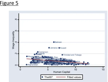
We know from above discussion that wage inequality in many developing countries

has deteriorated amid more international trade. In order to know whether human

capital accumulation, which is directly accrued through processes of trade, is guilty

of aggravating wage inequality in developing countries, the paper generates

predicted values of human capital by regressing them on FR (1999) predicted trade

shares. Figure 5 shows two graphs. First one illustrates a simple relation ship

Afghanistan

Angola

Albania

United Arab Emirates

Argentina Burundi

Benin Burkina FasoBangladesh

Bulgaria Bahrain Bahamas, The Belize Bolivia Brazil BarbadosBhutan Botswana

Central African Republic Chile China Cote d'Ivoire Cameroon Congo, Rep. Colombia Cape Verde

Costa RicaCuba

Cyprus

Dominican Republic Algeria

Ecuador

Egypt, Arab Rep.

Ethiopia Fiji Gabon Ghana Guinea Gambia, The Equatorial Guinea Guatemala

Hong Kong, China HondurasHaiti

Indonesia India

Iran, Islamic Rep. Iraq Jamaica Jordan Kenya Korea, Rep. Kuwait Liberia Libya Sri Lanka Lesotho Morocco Madagascar Mexico Myanmar Mongolia Mozambique Mauritania Mauritius Malawi Malaysia Namibia Nigeria NicaraguaNepal Oman Pakistan Panama Peru Philippines Papua New Guinea

Puerto Rico Paraguay Qatar Romania Rwanda Saudi Arabia Sudan Senegal SingaporeEl Salvador

Somalia Suriname

Swaziland Seychelles

Syrian Arab Republic

Togo

Thailand Tonga Trinidad and Tobago

Tunisia Turkey

Tanzania Uganda

Uruguay St. Vincent and the Grenadines

Venezuela, RB Samoa Yemen, Rep.

Yugoslavia, Fed. Rep.

South Africa ZambiaZimbabwe .0 5 .1 .1 5 .2 W a g e I n e q u a lit y

4 5 6 7 8

Human Capital(predicted from openness)

Fitted values Fitted values

Afghanistan Argentina BeninBangladesh Bahrain Bolivia Brazil _Barbados Botswana Central African Republic

Chile China Cameroon

Congo, Rep.

Colombia_{Costa Rica} Cyprus Dominican Republic Algeria

Ecuador Egypt, Arab Rep. Fiji Ghana

Gambia, TheGuatemala _{Hong Kong, China} Honduras

Haiti Indonesia India Iran, Islamic Rep. Iraq Jamaica Jordan Kenya Korea, Rep. Kuwait Liberia Sri Lanka Lesotho Mexico Myanmar Mozambique Mauritius Malawi Malaysia Nicaragua Nepal

Pakistan PeruPhilippinesPanama Papua New Guinea

Paraguay Rwanda SudanSenegal Singapore El Salvador Swaziland Syrian Arab Republic Togo

Thailand

Trinidad and Tobago Tunisia

Turkey Uganda

Uruguay Venezuela, RBSouth Africa Zambia Zimbabwe 0 .2 .4 .6 .8 W a g e I n e q u a lit y

0 5 10 15

Human Capital

Theil97 Fitted values

human capital do well apropos inequality. The second graph, where we predicted

human capital on FR trade shares, follows the opposite line and confirms that human

capital accumulation which is owed to global integration, carry augmented effects on

wage inequality. Now this leads to another question as to why would human capital

under liberalized trade work against wage equality in developing countries? The

answer is simple. Generally in most developing countries human capital is unevenly

distributed (Ravallion, 2003). Thomas, Wang and Fan (2000) and Domenech and

Castello (2002) have found out that Gini coefficient of the distribution of human

capital in Sub Saharan Africa and South Asia respectively, is the highest in the world.

Berthelemy (2004) came up with the same conclusion not only for Sub Saharan

Africa and South Asia but also for Middle East and North Africa (MENA). According to

Berthelemy (2004), the unequal distribution of income in these regions are due to

inequitable education policies of their respective governments who pay on average

much more attention to secondary and tertiary education than primary education.

Figure 5

One of the reasons for this biasness in education policies in these developing

countries towards higher education is the fact that elementary education has a very

limited direct role in determining growth rates. According to Barro (1999) the rate of

economic growth responds more to secondary or higher education levels rather than

elementary schooling. This is true because processes of growth are deeply linked

with higher education instead of primary education. For example, in developing

either highly qualified university graduates or those who have at least finished their

high school. The sole reason that India and China have been the haven for

international outsourcing and trade in contemporary times is because they have

managed to accumulate relatively educated and skilled human capital by investing

on higher education. It is expected that over the next five years, 3.3 million services

and industry jobs and $ 136 billion in wages will be outsourced only from United

States, while most of them finding their way to the Indian or Chinese Shores. Only in

India, on any given day in New Delhi, Bombay and Bangalore, the call goes for a new

call center recruits who are sufficiently educated to communicate in English and

have at least acquired a high school diploma. At least, as far as international trade is

concerned, it is quite evident that the Southern countries which are benefiting today

and which will benefit the most in near future are those who have transformed a

portion of their labor force into relatively skilled intensive by investing generously on

its higher education programs. Well, these countries are also the ones which have

been the fastest growing economies of recent times.

So it is no surprise that in order to be competitive in a race to the top, developing

countries generally have a tendency to invest in higher education at the cost of

primary education to achieve greater growth. Recently, Pakistan has also fallen for

this trap as its current education policy is skewed towards higher education, whereas

primary education is being overlooked. Only last year the government increased its

higher education budget to Rs 5 billion from a meager amount of Rs 800 million five

years ago - an increase of nearly 400 percent. For this year the government has

allocated double the amount of last year for higher education. Such a focus on

higher education is unprecedented in the history of this country. However allocation

of funds to primary education is in contrast with such heavy investments in higher

education since the budget for primary education has been increased by a meager

average of 4 percent for the last few years. Though, in coming years Pakistan will

definitely reap the fruits of its higher education focus and compete with other

developing countries in international markets for its cheap and skilled human capital,

relative wages of unskilled labor would decline amid increased international trade.

This apparent pro growth higher education policy of Pakistan at the cost of primary

education may very well be good for income generation but it definitely excludes the

poor and unskilled and will subsequently lead to increased wage and income

inequalities in the country.

In order to show how income inequalities increase with education inequality

Gregorio and Lee (1999) worked with a traditional model of human capital where the

level of earnings (Y) is accrued by an individual with S years of schooling:

………(9)





  

 s

j

j o

s Y r u

Y

1

) 1 log( log

log

where r_jis the rate of return to the jth year of schooling. The function can be

approximated by:

……….(10)

. log

logY_s  Y_o rSu

Whereas the distribution of earnings can be written as:

……….(11)

). , ( 2

) ( )

( )

( )

(logY Var rS r2Var S S2Var r rSCov r S

Var _s    

A sharp rise in educational inequalities Var(S) would unambiguously lead to higher

wage inequality in equation (11) if other variables are held constant. On the same

account, rise in wage inequality is a clear outcome if Var(r) is high. Here we know

that returns to higher education are greater than returns to primary education in

developing countries because of excess demand of skilled labor as rapid technology

diffusion amid trade liberalization takes place and skilled labor supply lags behind.

However, equation (11) also suggests that under the assumption of other things as

constant, if the covariance between the return to education and the level of

education is negative, an increase in schooling can reduce wage inequality. Well

return to education and average years of schooling (Teulings and Van Rens, 2002).

The negative value of Cov (r, S) suggest that as the relative supply of high skilled

workers go up and that of unskilled workers go down, the relative wages of skilled

labor decreases. Though Cov(r, S) gives some useful information apropos wage

inequality, the information can very well be misleading because movements in

relative wages are as much a function of ‘skilled labor demand’ as it is of skilled labor

supply. For example, through trade liberalization, there is a constant transfer of

technology in developing countries which increase the demand for skilled labor as

learning by doing takes place. If this increased demand for skilled labor is more than

its supply, there is a good possibility that wages of skilled labor rise instead of

plummeting. And if the wages of unskilled labor fail to rise simultaneously because

unskilled labor are in excess supply in developing countries, the wage inequality will

very well increase and the negative relationship between level of schooling and

returns to education Cov (r, S) might not hold at all. This fact is recognized by Dur

and Tuelings( 2002) when they admitted that in the Tinbergen’s (1975) famous race

between technology (skilled labor demand) and education (skilled labor supply),

technology has been a clear winner of recent times.

In short the key to equality of relative wages in developing countries do not lie as

much in Cov (r, S) but in the value of Var(S). Our discussion suggests that the

inequalities, which we witness today in developing countries, have two important

determinants. First there are significant inequalities in educational attainments.

Second, the processes of international trade transform these education inequalities

into wage inequalities by favoring the skilled labor.

Well to this effect, in order to solve for wage inequality in developing countries, the

respective governments need to increase the mean level of human capital through a

balanced education policy whereby primary education is given as much importance

as higher education. An equitable education policy will not only decrease Var(S), it

will also lead to a negative value of Cov(r, S) as the overall supply of low skilled and

Tuelings (2002) have called for subsidies to all levels of education as they argue that

the mean level of education gives rise to general equilibrium effects that reduce

wage inequality.

4. CONCLUSIONS:

The paper has found out that contrary to the claims of neo-classical paradigm,

openness does have significant effects on wage inequality. The empirical evidence

provided in the paper supports the argument that international trade is biased

towards skilled workers in developing countries and with an increase of trade after

liberalization, the wages of skilled workers are most likely to increase in South,

where as poor who are largely unskilled shall increasingly become the hostage of

such process.

This conclusion has some serious implications for the success of poverty reduction

strategies in developing countries because inequality is one of the two channels

through which poverty is affected. The newly adopted common wisdom that growth

always trickles down to decrease poverty if supplemented by certain relevant

development strategies e.g. micro finance schemes etc may be true but ignoring the

inequality part vis-a-vis poverty is a fatal mistake especially when pro poor growth

policies e.g. liberalization or opening up leads to increases in the formal variable

(inequality). The general perception among the right that inequality is never that

significant to offset pro poor growth effects is not true and has to be re-evaluated

also.

Recently, the World Bank has accepted this fact since its webpage4 _{on “Poverty”}

advices policy makers that poverty reduction and social development cannot be

achieved by focusing on growth strategies with out any understanding of their

effects on the distribution of income and wealth: “The benefits of growth for the

poor may be eroded if the distribution of income worsens. But policies that promote

better income distribution are not well understood; learning more about the impact

of policies on distribution should be high on the agenda”

All in all, it is apposite to conclude that more and more people might be able to live

above poverty line with increases in growth attributed to the so-called reform

process - thus showing some improvements regarding extreme poverty, but if

inequality is on rise more and more people are worse off and an increase of the gap

between have and have nots can not be defended with any academic jargon and is

definite welfare loss. Thus it becomes all more important to understand inequality

and its determinants. If free trade is guilty of increasing inequality among people or

societies, the process has to be sterilized against such a phenomenon.

The paper makes some suggestions to this effect. It tries to find those channels

through which liberalization causes wage inequality. In line with previous studies we

have found out that education is the key to explain the increasing gap in relative

wages. Though the paper supports the argument that those countries which starts

out with higher level of human capital do well on inequality front, it also suggests

that human capital which is accrued through the liberalization process is guilty of

unequal distribution of wages among skilled and unskilled labor. One explanation is

that governments in the developing countries invest in higher education at the cost

of primary education in order to accrue quicker benefits from processes of growth

and thus become prone to wage inequality after trade liberalisation.

The paper carries very important guide lines for policy makers. In order to neutralize

the unequal effects of trade, the focus of policy makers should be on education. The

countries, which have greater frequency of educated people, are in a better position

to benefit from international trade. However there is a caveat. Generally the

governments in developing countries tend to focus their education policy on higher

education in the anticipation that investments in higher education would accrue

faster dividends by exploiting the international business environment. Though they

cost of primary education. Since literature suggests that many developing countries

are guilty of promoting higher education at the cost of primary education, only a

limited segment of the society participates in activities emanating from international

trade, whereas the majority which is excluded is also be barred from the benefits of

growth and its processes (i.e., trade) at least in the short term. The cases in point are

China and India who have been the most prominent beneficiaries of international

trade. Though, both the countries are able to achieve high growth rates as their

relatively skilled and cheaper human capital ( a direct outcome of their higher

education focus) has utilized the recent surge of international outsourcing by

multinationals, they have suffered from increasing inequality because large portions

of the population are left out because they were illiterate and unskilled.

ACEMOGLU, Daron, JOHNSON, Simon and ROBINSON, James A., “The Colonial Origins of Comparative Development: An Empirical Investigation,” American Economic Review, Vol. 91, No. 5, 2001, pp. 1369-1401 http://emlab.berkeley.edu/users/chad/e236c_f04/ajr2001.pdf

AMANN, Edmund, ASLANINDIS, Nektarios, NIXSON, Fredrick, and WALTERS, Bernard, “Economic Growth and Poverty Alleviation: A Reconsideration of Dollar and Kraay,” Development Economic Discussion Papers, No. 0407, 2002.

http://les.man.ac.uk/ses/research/devpapers/Povertyconference%5B1%5D.pdf

ARBACHE, Jorge S., DICKERSON, Andy and GREEN, Francis, “Trade Liberalisation and Wages in Developing Countries,” Economic Journal, Vol. 114, No. 493, 2004, pp. 73-96

BARRO, Robert J., “Does an Income Gap Put a Hex on Growth’ Business Week, March 29, 1999

BEHRMAN, Jere R., BIRDSALL, Nancy, and SZEKELY, Miguel, “Pobreza, Desigualdad, y Liberalizacion Comercial y Financiera en America Latina.” Inter American Development Bank (IADB), Washington D.C, 2001 http://www.undp.org/rblac/liberalization/docs/capitulo3.pdf

BERTHELEMY, Jean-Claude, “To What Extent are African Education Policies Pro-Poor,” Unpublished, 2004

http://www.csae.ox.ac.uk/conferences/2004-GPRaHDiA/papers/5h-Berthelemy-CSAE2004.pdf

BOURGUIGNON, Francois and MORRISON, Christiasn., “Income Distribution, Development and Foreign Trade: A Cross Section Analysis,” European Economic Review, vol. 34, no. 6, 1999, pp. 1113-1132

CASTELLO, Climent, Maria Amparo and DOMENECH, Rafael, "Human Capital Inequality and Economic Growth: Some New Evidence,” Economic Journal, Vol. 112, 2002, pp. C187-C200

CHEN, Shaohua and RAVALLION, Martin, “Household Welfare Impacts of China’s Accession to the World Trade Organization,” World Bank Policy Research Working Paper 3040, 2003 www.econ.worldbank.org/files/26013_wps3040.pdf

COCKBURN, John, “Trade Liberalization and Poverty in Nepal: A Computable General Equilibrium Micro Simulation Analysis,” The Centre for the Study of African Economies Working Paper Series. Working Paper 170, 2002

http://www.bepress.com/csae/paper170

DE GREGORIO, Jose. and LEE, Jong-Wha, “Education and Income Distribution: New Evidence from Cross-Country Data,” Development Discussion Paper No. 714, Harvard Institute for International Development (HIID), 1999

http://www.hiid.harvard.edu/pub/pdfs/714.pdf

DOLLAR, David and KRAAY, Aart, “Trade, Growth, and Poverty,” Economic Journal, Vol. 114, pp. F22-F49, February 2004

DOLLAR, David and KRAAY, Aart, “Institutions, Trade and Growth,” Carnegie Rochester Conference on Public Policy, 2002

http://www.carnegie-rochester.rochester.edu/April02-pdfs/ITG2.pdf

DUR, Robert A. J. and TEULINGS, Coen N, “Education, Income Distribution and Public Policy,” Unpublished draft, Tinbergen Institute, 2002

http://www.iza.org/iza/en/papers/transatlantic/1_teulings.pdf

FISCHER, Ronald D., “The Evolution of Inequality after Trade Liberalization,” Journal of Development Economics, Vol. 66, 2001, p. 555-579.

FRANKEL, Jaffery and ROMER, David, “Does Trade Cause Growth?” American Economic Review, vol. 89, no. 3, 1999, pp 379-399.

FRIEDMAN, Jed, “Differential Impacts of Trade Liberalisation on Indonesia’s Poor and Non-Poor,” Conference on International Trade and poverty, Stockholm, October 20, 2000.

GOLDBERG, Pinelopi, Koujianou and PAVCNIK, Nina, “Trade, Inequality and Poverty: What Do We Know? Evidence From Recent Trade Liberalization Episodes in Developing Countries,” Conference Paper Brooking Trade Forum, 2004

http://www.econ.yale.edu/~pg87/brookings.pdf

HALL, Robert E., and CHARLES Jones, “Why do Some Countries Produce So Much More Output per Worker than others?” Quarterly Journal of Economics, Volume 114, 1999, pp. 83-116

HANSON, Gordon, and HARISSON, Ann, “Trade and Wage Inequality in Mexico,” Industrial and Labor Relations Review, Vol. 52, no. 2, 1999, pp. 271-288.

JAYASURIYA, Sisira, “Globalisation, Equity and Poverty: The South Asian Experience,” Annual Global Conference of GDN, Cairo, Egypt, 2002.

LEGOVINI, Avianna, BOUILLON, Cesar and LUSTIG, Nora, “Can Education Explain Income Inequality Changes in Mexico?” Inter-American development Bank (IADB), Washington D.C., 2001

LOFGREN, Hans, “Trade Reform and the poor in morocco: A Rural-Urban General Equilibrium Analysis of Reduced Protection,” TMD Discussion paper, IFPRI, Washington DC, No. 38, 1999

MURSHED, S. Mansoob, “Globalization is not always good: An Economists Perspective,” Tilburg Lustrum Conference, 2003

www.wider.unu.edu/conference/conference-2003-3/conference-2003-3-papers/Murshed-0307.pdf-

RAVALLION, Martin, “The Debate on Globalization, Poverty, and Inequality: Why Measurement Matters” World Bank Policy Research Working Paper 3038, Washington DC, 2003

http://econ.worldbank.org/files/26010_wps3038.pdf

RODRIK, Dani, SUBRAMANIAN, Arvind, and TREBBI, Francesco, “Institutions Rule: The Primacy of Institutions Over Geography and Integration in Economic Development,” Journal of Economic Growth, Vol. 9, no. 2, June 2004, pp. 131-165

ROSE, Andrew K., “Do WTO Members Have a More Liberal Trade Policy?” NBER Working Paper 9347, 2002

THOMAS, Vinod, WANG, Yan, and FAN, Xibo, “Measuring Education Inequality: Gini Coefficients of Education,” Mimeo, Banque Mondiale, 2000

http://econ.worldbank.org/files/1341_wps2525.pdf

TINBERGEN, Jan, Income Distribution: Analysis and Policies, Amsterdam: American Elsevier, 1975

TILAK, Jandhyala B. G., Education and its Relation to Economic Growth, Poverty and Income Distribution, World Bank: Washington D. C., 1989

WINTERS, L. Alan., “Trade Liberalization and Economic Performance: An Overview,” The Economic Journal, Vol. 114, 2004, pp. 4-21

WINTERS, L. Alan., “Trade Liberalisation and Poverty”, Discussion Paper No. 7, Poverty Research Unit, University of Sussex, UK, 2000

World Bank, A globalized Market – Opportunities and Risks for the Poor, Global Poverty Report, Washington D.C., 2001a.

World Development Report 2000/1, Attacking Poverty, 2001b

WOOD, Adrian, and RIDAO-CANO, Cristobal, “Skill, Trade and International Inequality,” Oxford Economic Papers, Vol. 5, No. 1, 1999, pp. 89-119.

http://www.ids.ac.uk/ids/bookshop/wp/wp47.pdf

APPENDIX 1.

Theil Indx 1 2 3 4 Theil Indx 1 2 3 4 lcopen hk disteq n 2 R

0.04 0.035 0.003 0.03 (2.58)* (2.6)* (1.8)** (1.82)*** -0.009 -0.008

(-2.1)** (-2.1)**

0.0002 0.0002 (0.35) (0.23)

70 70 114 114 0.11 0.11 0.03 0.02

Impen2a hk disteq n 2 R

-0.0003 -0.0003 -0.001 -0.001 (-0.15) (-0.12) (-0.5) (-0.49) -0.003 -0.004

(-0.7) (-0.8)

-0.0002 -0.0003 (-0.3) (-0.34)

58 58 72 72 0.01 0.01 0.005 0.0035

impen1o hk disteq n 2 R

0.0004 0.0004 0.0001 0.0001 (0.8) (0.95) (0.28) (0.27) -0.005 -0.005

(-0.9) (-1.13)

-0.0003 -0.0005 (-0.4) (-0.59)

59 59 73 73 0.03 0.02 0.006 0.001

Impen2r hk disteq n 2 R

0.002 0.002 0.0015 0.001 (2.6)* (2.67)* (1.5) (1.5) -0.007 -0.007

(-1.5) (-1.5)

0.00009 -0.0003 (0.1) (-0.3)

58 58 72 72 0.12 0.12 0.03 0.03

impen1m hk disteq n 2 R

0.0009 0.001 0.0005 0.0005 (1.2) (1.34) (0.69) (0.71) -0.005 -0.006

(-1.1) (-1.3)

-0.0003 -0.0005 (-0.3) (-0.6)

59 59 73 73 0.04 0.04 0.011 0.007

Tars1o hk disteq n 2 R

0.0005 0.0005 0.0005 0.0005 (1.8)*** (1.9)*** (1.7)*** (1.7)*** -0.007 -0.007

(-1.39) (-1.5)

-0.0001 -0.0004 (-0.04) ( 0.4)

59 59 73 73 0.07 0.07 0.04 0.04

Impen1a Hk disteq n 2 R

0.001 0.001 0.00001 -0.00001 (0.46) (0.48) (0.01) (0.001) -0.003 -0.004 -0.0005

(-0.71) (-0.9) (-0.6) -0.003

(-0.71)

59 59 73 73 0.02 0.01 0.18 0.0000

Tars1m Hk disteq n 2 R

-0.001 0.0002 0.0001 -0.0001 (-0.27) (0.36) (-0.17) (-0.18) -0.004 -0.005

(-0.73) (-0.36)

-0.0004 -0.0005 (-0.48) (-0.59)

59 59 73 73 0.02 0.015 0.005 0.0005

Impen1r Hk disteq n 2 R

0.0003 0.0002 -0.0007 -0.0007 (0.02) (0.09) (-0.45) (-0.5) -0.0033 -0.004

(-0.65) (-0.9)

-0.0005 -0.0005 (-0.5) (-0.6)

59 59 73 73 0.02 0.01 0.007 0.003

Tars1a Hk disteq n 2 R

-0.0008 -0.0004 -0.0009 -0.0006 (-0.5) (-0.29) (-0.7) (-0.5) -0.003 -0.004

(-0.6) (-0.9)

-0.0007 -0.0007 (-0.7) (-0.8)

59 59 73 73 0.02 0.43 0.01 0.003

Impen2o hk disteq n 2 R

0.0004 0.0005 0.0003 0.0003 (1.3) (1.3) (0.7) (0.75) -0.006 -0.005

(-1.1) (-1.19)

0.00001 -0.0002 (0.01) (-0.3)

58 58 72 72 0.04 0.04 0.009 0.008

Tars1r hk disteq n 2 R

0.002 0.003 0.003 0.003 (4.8)* (4.9)* (5.2)* (5.3)* -0.009 -0.01

(-2.2)** (2.3)**

0.0002 -0.0004 (0.35) (-0.6)

59 59 73 73 0.31 0.31 0.28 0.28

Impen2m hk disteq n 2 R

0.0002 0.0003 0.0002 0.0002 (0.4) (0.46) (0.31) (0.35) -0.004 -0.004

(-0.81) (-0.94)

-0.001 -0.0002 (-0.81) (-0.29)

58 58 72 72 0.01 0.01 0.003 0.001

Tars2o hk disteq n 2 R

0.0003 0.0003 0.00006 0.00006 (1.3) (1.4) (0.61) (0.6) -0.006 -0.006

(-1.2) (-1.3)

0.0001 -0.0007 (0.1) (-0.8)

57 57 70 70 0.04 0.05 0.01 0.005

-*, ** and *** denotes 1%, 5% and 10% level of significance respectively. ^ For variable descriptions please refer to appendix 1.

Table 1b: OLS Regression Results with different Specifications^

Theil Indx 1 2 3 4 Theil Indx 1 2 3 4

Tars2m -0.0001 -0.00006 -0.0001 -0.0001 (-0.21) (-0.13) (-0.3) (-0.27)

hk

disteq

n

2

R

-0.003 -0.003 (-0.54) (-0.71)

-0.0003 -0.001 (-0.34) (-0.77)

57 57 70 70 0.01 0.01 0.009 0.05

hk

disteq

n

2

R

-0.005 -0.006 (-1.00) (-1.2)

-0.0003 -0.0004 (-0.37) (-0.5)

55 55 70 70 0.05 0.05 0.05 0.05

Tars2a hk disteq n 2 R

-0.002 -0.001 -0.0007 -0.0005 (-1.3) (-1.14) (-0.8) (-0.62) -0.002 -0.003 -0.0008

(-0.47) (-0.77) (-0.9) -0.0008

(-0.8)

57 57 70 70 0.04 0.04 0.02 0.005

totgva hk disteq n 2 R

-0.0008 -0.0009 -0.001 -0.001 (-1.8)*** (-1.91)*** (-2.4)** (2.38)** -0.006 -0.006

(-1.16) (-1.31)

-0.0003 -0.0006 (-0.39) (-0.66)

55 55 70 70 0.08 0.07 0.08 0.076

Tars2r Hk disteq n 2 R

0.0017 0.0017 0.0002 0.0002 (3.8)* (3.9)* (1.19) (1.13) -0.008 -0.008

(-1.9)*** (-1.9)***

0.0003 -0.0007 (0.34) (-0.86)

57 57 70 70 0.228 0.227 0.029 0.018

totgvr hk disteq n 2 R

-0.0002 -0.003 -0.0005 -0.0006 (-0.48) (-0.52) (-1.02) (-1.04) -0.004 -0.0045

(-0.74) (-0.91) -0.0005 -0.0006 (-0.55) (-0.65)

55 55 70 70 0.02 0.018 0.022 0.015

tariffs Hk disteq n 2 R

-0.0015 -0.0015 -0.0006 -0.0007 (-1.2) (-1.2) (-0.4) (-0.5) -0.008 -0.008

(-1.5) (-1.6)

-0.0001 0.0003 (-0.1) (0.4)

59 59 82 82 0.05 0.05 0.005 0.003

owqi Hk disteq n 2 R

-0.038 -0.04 -0.049 -0.052 (-1.03) (-1.1) (-1.4) (-1.5) -0.005 -0.005

(-1.1) (-1.2) -0.0002 -0.0005 (-0.28) (-0.66)

59 59 72 72 0.04 0.04 0.03 0.02

owti Hk disteq n 2 R

-0.053 -0.055 -0.075 -0.077 (-0.9) (-1.0) (-1.4) (-1.4) -0.005 -0.005

(-1.13) (-1.2) -0.0003 -0.0006 (-1.13) (-0.8)

59 59 72 72 0.04 0.03 0.03 0.027

nontaro Hk disteq n 2 R

-0.0003 -0.0003 -0.0003 -0.0003 (-0.8) (-0.9) (-1.1) (-1.05) -0.004 -0.005

(-0.9) (-1.1)

-0.0004 -0.0007 (-0.5) (-0.7)

55 55 70 70 0.03 0.03 0.02 0.01

txtrg hk disteq n 2 R

0.096 0.089 0.19 0.165 (0.19) (0.18) (0.48) (0.43) -0.002 -0.002

(-0.26) (-0.29)

0.0006 0.0005 (0.51) (0.54)

40 40 46 36 0.01 0.006 0.01 0.005

nontarm hk disteq n 2 R

-0.0002 -0.0002 -0.0002 -0.0002 (-0.68) (-0.76) (-0.89) (-0.88) -0.0004 -0.005

(-0.49) (-1.02)

-0.004 -0.0006 (-0.49) (-0.7)

55 55 70 70 0.03 0.024 0.018 0.011

totgvo hk disteq n 2 R

-0.0006 -0.0006 -0.0009 -0.0009 (-1.3) (-1.42) (-1.8)** (-1.94) -0.005 -0.0058

(-1.0) (-1.15)

-0.0003 -0.0005 (-0.37) (-0.53)

55 55 70 70 0.05 0.05 0.05 0.05

nontara hk disteq n 2 R

-0.0002 -0.0002 -0.0003 -0.0003 (-0.8) (-0.85) (-1.09) (-1.06) -0.004 -0.005

(-0.8) (-1.03) -0.0005 -0.0007 (-0.5) (-0.74)

55 55 70 70 0.03 0.027 0.024 0.016

-*, ** and *** denotes 1%, 5% and 10% level of significance respectively. ^ For variable descriptions please refer to appendix 1.

Table 2a: IV Regression Results With Different Specifications^:

1 2 1 2 1 2

(2.25)* (1.14) (1.7)** (2.2)* (2.4)* (2.8)*

hk -0.008 hk -0.007 hk -0.009

(-2.12)* (1.4) (-2.14)*

F-test 3.5* 1.3 F-test 1.8 4.9* F-test 3.4* 8.2*

n 70 100 n 58 72 n 59 73

2

R 0.11 0.04 R2 _ _ R2 0.30 0.23

impen1o 0.0014 0.002 impen2a 0.007 0.01 tars2o 0.001 0.0004

(2.0)* (2.2)* (1.7)** (2.1)* (1.7)* (1.5)

hk -0.008 hk -0.006 hk -0.008

(-1.65)** (-1.2) (-1.6)

F-test 2.3** 5.1* F-test 1.7 4.5* F-test 1.8 2.2

n 59 73 n 58 72 n 57 70

2

R _ _ R2 _ _ R2 _ _

impen1m 0.002 0.003 impen2r 0.003 0.005 tars2m 0.001 0.001

(2.1)* (2.3)* (1.9)** (2.2)* (1.6) (1.5)

hk -0.009 hk -0.008 hk -0.009

(-1.7)** (-1.7)** (-1.5)

F-test 2.4** 4.9* F-test 2.2 4.5* F-test 1.6 2.4

n 59 73 n 58 72 n 57 70

2

R _ _ _R2 0.1 _ _R2 _ _

impen1a 0.007 0.01 tars1o 0.001 0.0012 tars2a 0.003 0.003

(1.91)** (2.2)* (2.1)* (2.8)* (1.39) (1.7)**

hk -0.005 hk -0.009 hk -0.004

(-0.9) (-1.8)** (0.87)

F-test 2.2 4.9* F-test 2.5* 6.16* F-test 1.2 2.8**

N 59 73 n 59 73 n 57 70

2

R _ R2 0.03 _ R2 _ _

impen1r 0.009 0.009 tars1m 0.002 0.002 tars2r 0.002 0.001

(1.7)** (1.9)** (1.9)** (2.1)* (1.96)* (1.2)

hk -0.012 hk -0.012 hk -0.009

(-1.6)** (-1.8)** (1.85)**

F-test 1.7 3.6** F-test 2.09 4.5* F-test 2.3** 1.5

n 59 73 n 59 73 n 57 70

2

R _ R2 _ _ R2 0.21 _

impen2o 0.001 0.002 tars1a 0.005 0.005 tariffs -0.005 -0.016

(1.8)** (2.3)* (1.7)** (2.1)* (-0.72) (-1.1)

hk -0.007 hk -0.003 hk -0.014

(-1.5) (-0.5) (-1.12)

F-test 1.9 5.1* F-test 1.7 4.31* F-test 0.92 1.38

n 58 72 n 59 73 n 59 78

2

R 0.006 _ R2 _ _ R2 _ _

- * and ** denote significance at 5% and 10% level. ^ For variable descriptions please refer to appendix 1.

1 2 1 2

owti -0.31 -0.26 totgvr -0.004 -0.004

(-234)* (-1.7)** (-1.7)** (-2.1)*

hk -0.004 hk -0.008

(-1.56) (-1.2)

F-test 3.3* 3.4* F-test 1.7 4.4*

n 73 109 n 55 70

2

R 0.08 0.01 R2 _ _

txtrg 3.34 3.05 owqi -0.23 -0.39

(1.40) (1.38) (-0.88) (-1.3)

hk 0.014 hk -0.008

(0.74) (-1.3)

F-test 2.2 3.9 F-test 0.8 1.5

n 49 66 n 59 72

2

R _ _ R2 _ _

totgvo -0.002 -0.002 nontaro -0.002 -0.002

(2.1)** (-2.5)** (-1.6)** (2.1)*

hk -0.009 hk -0.013

(-1.5) (-1.5)

F-test 2.6*** 6.6* F-test 1.6 4.5*

n 55 70 n 55 70

2

R _ _ R2 _ _

totgvm 0.002 -0.002 nontarm -0.002 -0.002

(-2.1)* (-2.6)* (-1.6) (2.02)*

hk -0.009 hk -0.015

(-1.5) (-1.5)

F-test 2.6** 6.6* F-test 1.42 4.1*

n 55 70 n 55 70

2

R _ _ R2 _ _

totgva -0.002 -0.002 nontara -0.003 -0.002

(-2.2)* (-2.6)* (-1.2) (-1.9)**

hk -0.009 hk -0.018

(-1.7)** (-1.3)

F-test 2.7** 6.8* F-test 0.9 3.5**

n 55 70 n 55 70

2

R _ _ _R2 _ _

- * and ** denote significance at 5% and 10% level. ^ For variable descriptions please refer to appendix 1.

DATA AND SOURCES:

Black: Black Market Premium, Year: 1985. Source: Rose (2002).

Disteq: Distance from Equator of capital city measured as abs (Latitude)/90. Source: Rodrik, Subramanian & Trebbi (2002)

heritage: Heritage Foundation Index, Source: Rose (2002).

hk: Average Schooling Years in the total population at 25,Year: 1999. Source: Barro R & J. W.

Lee data set, http://post.economics.harvard.edu/faculty/barro/data.html

hyr: Average Years of Higher Schooling in the Total Population at 25, Year: 1999.

Source: Barro R & J. W. Lee data set,

http://post.economics.harvard.edu/faculty/barro/data.html

Impen1o: Import Penetration: overall, 1985. Source: Rose (2002).

Impen1m: Import penetration: Manufacturing, 1985. Source: Rose (2002).

Impen1a: Import Penetration: Agriculture, 1985. Source: Rose (2002).

Impen1r: Import Penetration: Resources, 1985. Source: Rose (2002).

Impen2o: Import Penetration: overall, 1982. Source: Rose (2002).

Impen2m: Import penetration: Manufacturing, 1982. Source: Rose (2002).

Impen2a: : Import Penetration: Agriculture, 1982. Source: Rose (2002).

Impen2r: Import Penetration: Resources, 1982. Source: Rose (2002).

Lcopen: Natural logarithm of openness. Openness is given by the ratio of (nomnal) imports plus exports to GDP (in nominal US dollars), Year: 1985. Source: Penn World Tables, Mark 6.

Logfrankrom: Natural logarithm of predicted trade shares computed following Frankel and Romer (1999) from a bilateral trade equation with ‘pure geography’ variables. Source: Frankel and Romer (1999).

Nontaro: Non- Taiff Barriers Coverage: Overall, 1987. Source: Rose (2002).

Nontarm: Non- Taiff Barriers Coverage: manufacturing, 1987. Source: Rose (2002).

Nontara: Non- Taiff Barriers Coverage: agriculture, 1987. Source: Rose (2002).

Nontarr: Non- Taiff Barriers Coverage: resources, 1987. Source: Rose (2002).

Open80: Sachs and Warners (1995) composite openness index. Source: Rose (2002).

Owti: Tariffs on Intermediate and Capital Goods, 1985. Source: Rose (2002)

Tars1o: TARS Trade Penetration: overall, 1985. Source: Rose (2002).

Tars1m: TARS Trade Penetration: manufacturing, 1985. Source: Rose (2002).

Tars1a: TARS Trade Penetration: agriculture, 1985. Source: Rose (2002).

Tars1r: TARS Trade Penetration: resources, 1985. Source: Rose (2002).

Tars2o: TARS Trade Penetration: overall, 1982. Source: Rose (2002).

Tars2m: TARS Trade Penetration: manufacturing, 1982. Source: Rose (2002).

Tars2a: TARS Trade Penetration: agriculture, 1982. Rose (2002).

Tars2r: TARS Trade Penetration: resourses, 1982. Rose (2002).

Tariffs: Import Duties as percentage imports, Year:1985. Source: World Development Indicators (WDI), 2002.

Theil97: UTIP-UNIDO Wage Inequality THEIL Measure - calculated based on UNIDO2001 by UTIP, Year: 1997. Source: University of Texas Inequality Project (UTIP)

http://utip.gov.utexas.edu.

Totgvo: Weighted Average of Total Import Charges: overall, 1985. Source: Rose (2002)

Totgvm: Weighted Average of Total Import Charges: manufacturing, 1985. Source: Rose (2002)

Totgva: Weighted Average of Total Import Charges: agriculture, 1985. Source: Rose (2002)

Totgvr: Weighted Average of Total Import Charges: resourses, 1985. Source: Rose (2002)

APPENDIX 3:

LIST OF COUNTRIES Afghanistan (1988)

Albania (1997) Algeria (1997)

Angola (1993) Argentina (1996) Armenia (1997) Azerbaijan (1994) Bahamas, The (1990) Bahrain (1992) Bangladesh (1990) Barbados (1997) Belize (1992) Benin (1981) Bhutan (1989) Bolivia (1997) Bosnia (1990) Botswana (1997) Brazil (1994) Bulgaria (1997) Burkina Faso (1981) Burundi (1990) Cameroon (1997) Cape Verde (1993) Central African Republic (1993) Chile (1997) China (1985) Colombia (1997)

Congo, Rep. (1988) Costa Rica (1997) Cote d'Ivoire (1997) Croatia (1994) Cuba (1988) Cyprus (1997)

Dominican Republic (1985) Ecuador (1997)

Egypt, (1997) El Salvador (1997) Equatorial Guinea (1990) Eritrea (1988) Ethiopia (1997) Fiji (1997) Gabon (1994)

Gambia, The (1981) Ghana (1995)

Guatemala (1997) Haiti (1988) Honduras (1994) Hong Kong, China (1997) India (1997)

Indonesia (1997) Iran, Islamic Rep (1993) Iraq (1985)

Jamaica (1990) Jordan (1997) Kenya (1997) Korea, Rep. (1997) Kuwait (1997)

Kyrgyz Republic (1994) Latvia (1997) Lesotho (1994) Liberia (1985) Libya (1980) Lithuania (1997) Macao, China (1997) Macedonia, FYR (1996) Madagascar (1988) Malawi (1997)

Malaysia (1997) Mauritania (1978) Mauritius (1997)

Mexico (1997) Moldova (1994) Mongolia (1994) Morocco (1997) Mozambique (1994) Myanmar (1997) Namibia (1994)

Nepal (1996) Nicaragua (1985) Nigeria (1994) Oman (1997)

Pakistan (1996) Panama (1997) Papua New Guinea (1989) Paraguay (1991) Peru (1994) Philippines (1997) Puerto Rico (1997) Qatar (1994)

Romania (1994) Rwanda (1985) Saudi Arabia (1989)

Senegal (1997) Seychelles (1988) Singapore (1997) Slovak Republic

(1997)

Slovenia (1997) Somalia (1986) South Africa (1997)

Sri Lanka (1994) St. Vincent and the

Grenadines (1994) Sudan (1972) Suriname (1993)

Swaziland ((1994) Syria (1997) Togo (1981) Thailand (1994) Tonga (1994) Trinidad and Tobago (1994)

Tunisia (1997) Turkey (1997) Taiwan (1997) Tanzania (1990) Uganda(1988) Ukraine (1997) United Arab Emirates (1985)

Ukraine (1997) Uruguay(1997) Venezuela (1994) Western Samoa (1972) Yemen (1986)