The Relation between Absences and Grades: A Statistical Analysis

Munich Personal RePEc Archive

The Relation between Absences and

Grades: A Statistical Analysis

Leon, Costas

18 February 2018

Online at

https://mpra.ub.uni-muenchen.de/84655/

The Relation between Absences and Grades: A Statistical Analysis

Costas Leon1

Abstract

The paper investigates the relation between absences and grades by employing statistical modelling and using data from a private hospitality school. The obtained parameters estimates verify the assumption that there exists an inverse relationship between absences and grades. It is shown that one unit increase in normalized absences leads to 0.814 units decrease in the average class grade. Further, a dynamic interaction between absences and grades is examined by means of a VAR model. No evidence that the links between absences and grades are propagated over time is found. The system has no memory: each term and / or course defines its own dynamics which is not spread over other terms and / or other courses.

Keywords: Students' performance, tardiness, absences, education, GARCH models, VAR models.

1. Introduction

The relation between absences and students performance is one of the most discussed topics in Education at all levels. Intuition and common sense as well as academic research suggest an inverse relation between absences and students' performance as this reflected on their grades. In this context, inverse relation is understood as, as long as absences increase (decrease), school performance decrease (increase). Studies from several researchers such as, for instance, Mizell (1987), Ligon and Jackson (1988), Cuellar (1992), Escourt (1986), Ediger (1987), all cited by Weade in her Master's thesis (2004), have shown that tardiness (late arrival in the classroom) and/or absences are known factors which contribute to failure, dropout and lower academic performance. In the same thesis, Weade (op.cited) has shown that unexcused absences and GPA are negatively correlated, as it is evidenced by a negative Pearson correlation coefficient equal to -0.519. Similar results have also been observed by Silvestri (2003), Callahan (1993), Hammen and Keeland (1994). In general, all the relevant literature shows an inverse relation between absences and performance which is also independent of the subject of study (LeBlanc III, 2005).

The vast majority of researchers employ statistical tools such as descriptive statistics, the correlation coefficient and/or classical multivariate regression analysis. The present paper attempts to investigate the relation between class attendance and students performance by employing relatively advanced statistical modelling. In particular, the main focus on the paper is the quantification of the response of

grades to the students’ absences using relevant statistical data obtained from the records of a private

hospitality school2_{. The advanced modelling techniques in the present paper refer to the use of GARCH}

models (Engle, 1982) as a potential tool for measuring volatility clustering, possibly existing in educational time series data, and, also, to the use of a Vector Autoregression Model (Lütkepohl and Krätzig, 2004) as a device of measuring dynamic interaction between grades and absences over time.

The paper is organized as follows: In Section 1, a descriptive analysis of the variables of consideration is presented. In Section 2, a series of models is employed in order to arrive at a statistically admissible and reliable model. The significance of relevant diagnostic and misspecification tests, as well as estimates of parameters of interest, are also presented here. In Section 3, the obtained results are discussed and future research paths are suggested. Diagrams, graphs and other important tools of analysis are presented in the Appendix under the generic term Figure.

1 _{Independent researcher. Email: [email protected].}

2. Statistical Analysis 2.1 Descriptive Statistics

Data and Variables

In this paper, the data refer to the period winter 2013 - fall 2014 (8 three-month terms) and concern the courses of Microeconomics, Macroeconomics, Mathematics, Calculus and Statistics. There are 35 observations in total, from which the first 18 refer to 2013 and the remaining 17 refer to 2014. The

data have been obtained from the schools’ management system, based on the class record book and

the examination papers. The variables under consideration are: the number of students, absences and grades.

Number of Students

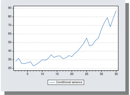
The analysis of the data shows that no change in the mean number of students over the two-year period is observed. However, the volatility increases significantly. It is observed that unconditional volatility, measured by the unconditional variance, in 2014 is almost double of the volatility in 2013: variance (2014) = 59 whereas variance (2013) = 29.15. Conditional variance, modelled by a GARCH (0,1) process, is statistically significant at 10% significance level. However, the effect of volatility clustering, measured by the GARCH model, is rather marginal and, therefore, the normality hypothesis of the number of students cannot be rejected at 5% significance level. See Figures 1a - 1d.

Absences

The total number of absences depend on the number of students enrolled in a class. Therefore, a measure independent of the number of students is needed. This leads to the introduction of the concept of normalized absences. It is defined as: Number of Absences / (Number of Students x Number of Contact Hours). In the school the contact hours are 40. Throughout the paper, several diagnostics and misspecification tests are involved in the various models proposed. Indicatively, for the detection of the order of autocorrelation the Hannan - Quinn criterion (1979) is used, for the unit roots test the Dickey-Fuller test (1979) with the MacKinnon, Haug Michelis (1999) critical values is employed while for normality the Jarque-Berra test is used. Several other tests employed in the paper, such as the Chow test, the Ramsey misspecification test, the Breusch-Pagan-Godfrey heteroskedasticity test, the Lagrange multiplier serial correlation test or, where appropriate, the Durbin-Watson test for first order autocorrelation, can be found in introductory econometrics texts.

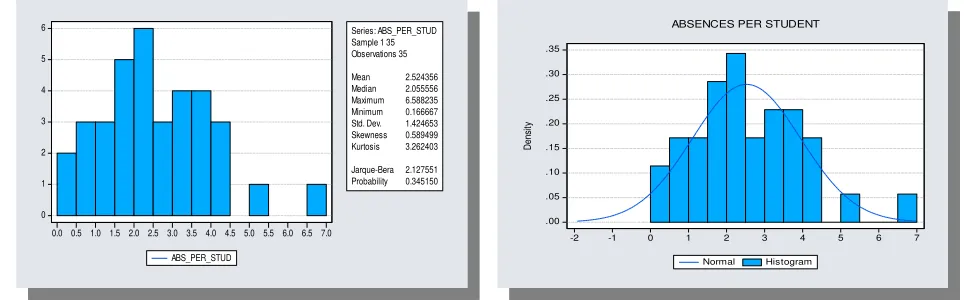
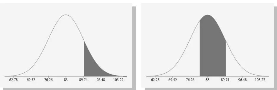
From the descriptive analysis, it is observed that the distribution of normalized absences is positively asymmetric. This is attributed to exceptional number of absences in some courses, as, for example, in Mathematics in winter 2013. It also turns out from the analysis that there is no change in the average number of normalized absences over the two-year period under consideration. This finding is supported by relevant diagnostic tests, that is, no ARIMA and/or GARCH processes are detected, no autocorrelation, heteroskedasticity and lack of normality are present and no structural break takes place over the two-year period under consideration. Therefore, we may safely assume that normalized absences follow a white noise process with mean 6.3 and standard deviation 3.56. The mean value of 6.3 suggests that, on average, 6.3% of the taught hours are missing due to absences. The standard deviation, in combination to the fact that the theoretical distribution is normal, implies that the probability of normalized absences, being between 2.74% and 9.86%, is approximately equal to 68%. Details of the analysis are presented in Figures 2a - 2k.

Grades

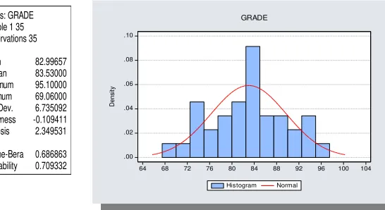
model may be safely considered statistically admissible. Given these results, the theoretical probabilities of the average class grades are also estimated. They are as follows: probability of grade A=14.95%, probability of grade B=52.24%, probability of grade C=30.12%, probability of grade D=2.66%, probability of grade < D=0.03%. More details are presented in Figures 3a-3k.

2.2 Statistical Modelling of the Relation between Absences and Grades 2.2.1 Response of Grades to Absences: the Correlation Coefficient

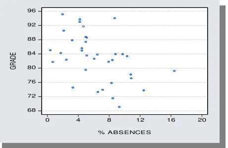
In the following, where absences are mentioned, they are understood as normalized absences. A first measure of the relation between grades and absences can be obtained by the correlation coefficient which is a measure of linear association between these two variables. With the given data, the correlation coefficient equals -0.45, a moderate inverse relation between absences and grades. This is expected, since absences partly but significantly affect class performance, as intuition, common sense and existing research have shown.

2.2.2 Response of Grades to Absences: Searching for a Suitable Statistical Model

The models below attempt to quantify the relationship between grades and absences. Model 1, estimated by maximum likelihood, is an exponential GARCH (1,1) model which shows that there is no GARCH process in the data. Therefore, a model without GARCH process is estimated by OLS. This is the Model 2a which shows that a deterministic trend is statistically insignificant. Because of the insignificance of the trend, the deterministic trend is removed and the next Model 2b is estimated. This model does not show autocorrelation, heteroskedasticity, AR-GARCH effects, or lack of normality.

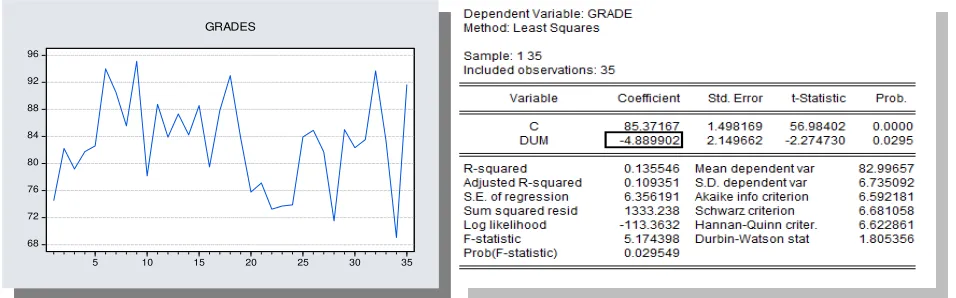
This is a better model than Model 2a but it displays instability in the beginning of 2014 as the Chow test shows. Therefore, an introduction of a dummy variable, with values 0 for 2013 and 1 for 2014, is added to the model. This is a new model, the Model 2c, which, based on all diagnostic tests, is statistically admissible. The estimates are: 4 .5 1 0 .0 1x

fo r 2 0 1 3

y



e

fo r 2 0 1 4

y



e

model to the data, as it is measured by the coefficient of multiple determination R square, is 32%, suggesting that absences explain 32% of the grades, whereas the remaining 68% is not captured by the model. To make the interpretation of this model easier, a linear model, with a dummy variable introduced as above, is estimated as an alternative to Model 2c. This is an almost statistically equally accepted model and it is the final model on which the interpretation of the relation between grades and absences is based.

The estimated models are:

9 0 .3 3

0 .8 1 4 fo r 2 0 1 3

y





x

y



8 5 .8 1 0 .8 1 4 fo r 2 0 1 4



x

is as follows:

Interpretation of the linear model for 2013:

If normalized absences increase (decrease) by 1 unit, then the grade will decrease (increase) on average by 0.814 units, provided that all implicitly considered variables included in the intercept remain constant. If there were no absences (x=0), then the average grade would be 90.33.

Interpretation of the linear model for 2014:

If normalized absences increase (decrease) by 1 unit, then the grade will decrease (increase) on average by 0.814 units, provided that all implicitly considered variables included in the intercept remain constant. If there were no absences (x=0), then the average grade would be 85.81.

2.2.3 Response of Grades to Absences: Dynamic Interaction

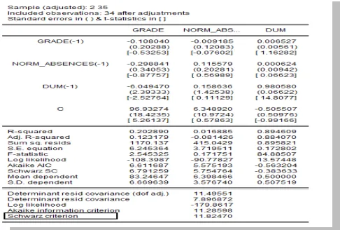
There is a theoretical possibility that the effects of grades and absences are propagated over time due to conscious or subconscious memory effects: the students may remember the relation between grades and absences from their own experience and, also, lectures may remember the same relation from their own experience too. For this purpose, a dynamic model has been built and estimated in order to investigate to which extent grades and absences interact over time. The model employs an impulse mechanism (the error term) and a propagation mechanism (a time lag structure). The precise structure of these two mechanisms has been found from the estimates and the diagnostics of a Vector Autoregression Model (VAR). The estimates, on the basis of several lag selection criteria (see, for example, Akaike, 1974 or Hannan - Quinn, 1979), suggest a model with one time lag and white noise residuals. The model, without the dummy variable, has the functional form:

1 1

11 12 1

1 2

21 22

t t t

t t

t t t

a

a

y

y

u

a

a

x

x

u

 







 



 





 

 









 





 







 



t

y

Ay

u

y

grades and absences,

u

A

The experimentation with this model, by means of impulse-response functions, shows that grades and absences do not dynamically interact over time. Put it differently, grades and absences do not

“remember” each other over time. A possible interpretation might be that the lecturer is not biased

against students at any current term and at any current course because of students' absences at any

course at the previous term. Also, students do not “remember” the effect of their previous absences

on their current grades. The system has no memory: absences and grades are not dynamically linked. Each term and / or course defines its own dynamics which is not spread over other terms and / or other courses. See Figures 4q-4u.

3. Conclusion and Suggestions for Further Research

The present paper is an attempt to quantify the relation between the relation of absences and average class performance by means of statistical modelling. The models employed have been thoroughly tested for statistical pitfalls by means of appropriate diagnostic and misspecification tests. In this context, the obtained estimates may be considered quite reliable. The finally chosen models (Model 2c and the linear model) establish that the relation between grades and absences is statistically very significant and verify the common intuition. The findings are also consistent with the existing literature in that absences affect negatively the grades: one unit increase in normalized absences leads to 0.814 units decrease in the average class grade. Although absences do play a role in class performance, they contribute only by 32% to the explanation of the class grades. It must, however, be noted that, given that the models are statistically well-behaved, the addition of other explanatory variables does not alter the quantitative relation between grades and absences. That is, it is expected that, again, one unit increase in normalized absences leads to 0.814 units decrease in the average class grade. This stability is an important property of the established statistical adequacy of the employed models. Further, the evidence of no interaction between grades and absences over time may imply that the lecturer is not biased against students at any current term and at any current course because of students' absences at any course at a previous term. The findings of the present paper strongly suggest the formulation of attendance policies which take into consideration the relation between grades and academic performance more effectively.

The above exposed analysis may also be enriched with some additional elements. For example, it is reasonable to assume that the background of the students before their admission to the school is a very important explanatory factor of their performance in the school. Therefore, data referring to the students' background and introduced in an appropriate statistical model, may significantly enhance the explanatory power of the analysis.

References

Akaike, H., (1974). A new look at the statistical model identification. IEEE Transactions on Automatic

Control, 19 (6): 716–723.

Callahan, S. (1993, November). Mathematics placement at Cottey College. Paper presented at the

annual conference of the American Mathematical Association of Two-Year Colleges, Boston, MA. (ERIC Document Reproduction Service No. ED 373813).

Cuellar, A. (1992). From dropout to high achiever: An understanding of academic excellence through

the ethnography of high and low achieving secondary school students (BBB27814). San Diego State

University, CA. Imperial Valley Campus. Institute of Borders Studies.

Dickey, D.A. and Fuller, W.A., (1979). Distributions of the estimators for autoregressive time series

with a unit root. Journal of the American Statistical Association, 74: 427-431.

Ediger, M. (1987). School Dropouts, Absenteeism, and Tardiness. (CGO019750). Counseling and

Personnel Services.

Engle, R.F., (1982). Autoregressive conditional heteroscedasticity with estimates of variance of United

Kingdom inflation. Econometrica, 50: 987-1008.

Estcourt, C. et al. (1986). Chronic absentee committee report at Centennial High School (CGO020358).

Counseling and Personnel Services.

Hammen, C. S. and Kelland, J. L. (1994). Attendance and grades in a human physiology course.

Advances in Physiology Education, 12 (1), S105-S108.

Hannan, E. J. and Quinn, B. G., (1979). The determination of the order of an autoregression. Journal

of Royal Statistical Society, 41: 190-195.

Jarque, C.M., and Bera, A.K., (1980), Efficient tests for normality, homoscedasticity and serial

independence of regression residuals. Economics Letters, Volume 6, Issue 3: 255-259

LeBlanc III P., H., (2005, April). The relationship between attendance and grades in the college

classroom. Paper presented at the 17th Annual Meeting of the International Academy of Business

Disciplines, Pittsburgh Pennsylvania.

Ligon, G. and Jackson, E. E. (1988). Why secondary teachers fail students (TMO13879).

Lütkepohl H. and Krätzig M. (2004). Applied Time Series Econometrics. Cambridge University Press.

MacKinnon, J. G., Haug, A. A., Michelis, L. (1999). Numerical distribution functions of likelihood ratio

tests for cointegration. Journal of Applied Econometrics, 14: 563-577.

Mizell, M. H. (1987). A guide for the identification of a student meriting special dropout

prevention initiatives (CG019711). Counseling and Personnel Services.

Silvestri, L. (2003). The effect of attendance on undergraduate methods course grades.

Education, 123 (3), 483-486.

Stradford, C. W. (1993). Implementation of a rural program to reduce the drop-out rate of 9th

APPENDIX

Figure 1a: No of Students. Figure 1b: Conditional Variance of No of

Students. 0 4 8 12 16 20 24 28

5 10 15 20 25 30 35

No of STUDENTS

0 4 8 12 16 20 24 28

5 10 15 20 25 30 35

No of STUDENTS

20 30 40 50 60 70 80 90

5 10 15 20 25 30 35 Conditional variance 20 30 40 50 60 70 80 90

5 10 15 20 25 30 35 Conditional variance

Figure 1c: Histogram and Descriptive Measures Figure 1d: Histogram and the Corresponding

Theoretical Normal Distribution.

0 1 2 3 4 5 6 7 8 9

2.5 5.0 7.5 10.0 12.5 15.0 17.5 20.0 22.5 25.0 27.5

Series: NO_STUDENTS Sample 1 35 Observations 35

Mean 12.31429 Median 11.00000 Maximum 26.00000 Minimum 4.000000 Std. Dev. 6.506881 Skewness 0.455217 Kurtosis 2.095223

Jarque-Bera 2.402619 Probability 0.300800

.00 .02 .04 .06 .08 .10

-5 0 5 10 15 20 25 30

Histogram Normal D e n si ty

No of STUDENTS

.00 .02 .04 .06 .08 .10

-5 0 5 10 15 20 25 30 Histogram Normal D e n si ty

No of STUDENTS

Figure 2a: Absences for all Taught Subjects. Figure 2b: Histogram of Absences and

Descriptive Measures. 0 20 40 60 80 100 120

5 10 15 20 25 30 35

ABSENCES 0 20 40 60 80 100 120

5 10 15 20 25 30 35

ABSENCES 0 1 2 3 4 5 6 7 8

0 10 20 30 40 50 60 70 80 90 100 110 120 ABSENCES

Series: ABSENCES Sample 1 35 Observations 35 Mean 31.11429 Median 23.00000 Maximum 112.0000 Minimum 2.000000 Std. Dev. 25.74167 Skewness 1.323218 Kurtosis 4.382025 Jarque-Bera 12.99903 Probability 0.001504

0 1 2 3 4 5 6 7 8

0 10 20 30 40 50 60 70 80 90 100 110 120 ABSENCES

Figure 2c: Histogram and Kernel: Figure 2d: Box-Plot of Absences:

Unusually many absences: Mathematics, Positively Asymmetric Distribution.

Winter 2013. .000 .004 .008 .012 .016 .020 .024

-20 0 20 40 60 80 100 120 140

Histogram Kernel D en si ty ABSENCES .000 .004 .008 .012 .016 .020 .024

-20 0 20 40 60 80 100 120 140 Histogram Kernel D e n si ty ABSENCES 0 2 0 4 0 6 0 8 0 1 0 0 1 2 0

ABSENCES 0 2 0 4 0 6 0 8 0 1 0 0 1 2 0

AB S E NC E S

Figure 2e: Absence per Student for all Taught Figure 2f: Absence for all Taught Subjects.

Subjects. 0 1 2 3 4 5 6

0.0 0.5 1.0 1.5 2.0 2.5 3.0 3.5 4.0 4.5 5.0 5.5 6.0 6.5 7.0

ABS_PER_STUD

Series: ABS_PER_STUD Sample 1 35 Observations 35

Mean 2.524356

Median 2.055556

Maximum 6.588235

Minimum 0.166667

Std. Dev. 1.424653 Skewness 0.589499 Kurtosis 3.262403

Jarque-Bera 2.127551 Probability 0.345150

0 1 2 3 4 5 6

0.0 0.5 1.0 1.5 2.0 2.5 3.0 3.5 4.0 4.5 5.0 5.5 6.0 6.5 7.0 ABS_PER_STUD

Series: ABS_PER_STUD Sample 1 35 Observations 35 Mean 2.524356 Median 2.055556 Maximum 6.588235 Minimum 0.166667 Std. Dev. 1.424653 Skewness 0.589499 Kurtosis 3.262403 Jarque-Bera 2.127551 Probability 0.345150

.00 .05 .10 .15 .20 .25 .30 .35

-2 -1 0 1 2 3 4 5 6 7

Normal Histogram

D

en

si

ty

ABSENCES PER STUDENT

.00 .05 .10 .15 .20 .25 .30 .35

-2 -1 0 1 2 3 4 5 6 7 Normal Histogram

D

en

si

ty

ABSENCES PER STUDENT

Figure 2g: Normalized Absences for all Taught Figure 2h: Stability of the Estimated Constant

by Subjects. By means of the Cumulative Sum of Squares.

0 4 8 12 16 20

5 10 15 20 25 30 35

NORMALIZED ABSENCES 0 4 8 12 16 20

5 10 15 20 25 30 35

NORMALIZED ABSENCES -0.4 0.0 0.4 0.8 1.2 1.6

5 10 15 20 25 30 35 CUSUM of Squares 5% Significance

-0.4 0.0 0.4 0.8 1.2 1.6

Figure 2i: Histogram of Normalized Absences Figure 2j: Histogram of Normalized Absences

and Descriptive Measures. and the Theoretical Normal Distribution.

0 1 2 3 4 5 6

0 1 2 3 4 5 6 7 8 9 10 11 12 13 14 15 16 17

Series: NORM_ABSENCES Sample 1 35 Observations 35 Mean 6.310891 Median 5.138889 Maximum 16.47059 Minimum 0.416667 Std. Dev. 3.561633 Skewness 0.589499 Kurtosis 3.262403 Jarque-Bera 2.127551 Probability 0.345150

.00 .02 .04 .06 .08 .10 .12 .14 .16

-6 -4 -2 0 2 4 6 8 10 12 14 16 18

Histogram Normal

D

en

si

ty

NORMALIZED ABSENCES

.00 .02 .04 .06 .08 .10 .12 .14 .16

-6 -4 -2 0 2 4 6 8 10 12 14 16 18 Histogram Normal

D

e

n

si

ty

NORMALIZED ABSENCES

Figure 2k: No change over time. No ARIMA and/or GARCH processes are detected. No autocorrelation, heteroskedasticity and lack of normality are present. No structural break. The process is white noise.

-8 -4 0 4 8 12

0 5 10 15 20

5 10 15 20 25 30 3 5

Residual Actual Fitted

-8 -4 0 4 8 12

0 5 10 15 20

5 10 15 20 25 30 35

Res idual A c tual Fitted

Figure 3a: Grades over Time. Figure 3b: Structural Break in the Intercept.

68 72 76 80 84 88 92 96

5 10 15 20 25 30 35

GRADES

68 72 76 80 84 88 92 96

5 10 15 20 25 30 35

GRADES

Figure 3c: Serial Correlation and Heteroskedasticity Tests.

Breusch-Godfrey Serial Correlation LM Test:

F-statistic 0.005903 Prob. F(2,31) 0.9941

Obs*R-squared 0.013325 Prob. Chi-Square(2) 0.9934

Heteroskedasticity Test: Breusch-Pagan-Godfrey

F-statistic 0.898368 Prob. F(1,33) 0.3501 Obs*R-square 0.927563 Prob. Chi-Square(1) 0.3355 Scaled explained SS 0.535751 Prob. Chi-Square(1) 0.4642

Figure 3d: Stability of the Intercept after the Introduction of the Dummy Variable.

-12 -8 -4 0 4 8 12

20 21 22 23 24 25 26 27 28 29 30 31 32 33 34 35 CUSUM 5% Significance

-12 -8 -4 0 4 8 12

20 21 22 23 24 25 26 27 28 29 30 31 32 33 34 35 CUSUM 5% Significance

Figure 3e: Histogram of Grades. Figure 3f: Histogram and the Theoretical

Normal Distribution of Grades.

0 1 2 3 4 5 6 7 8 9

70 75 80 85 90 95

Series: GRADE Sample 1 35 Observations 35 Mean 82.99657 Median 83.53000 Maximum 95.10000 Minimum 69.06000 Std. Dev. 6.735092 Skewness -0.109411 Kurtosis 2.349531 Jarque-Bera 0.686863 Probability 0.709332

.00 .02 .04 .06 .08 .10

64 68 72 76 80 84 88 92 96 100 104

Histogram Normal

D

e

n

si

ty

GRADE

.00 .02 .04 .06 .08 .10

64 68 72 76 80 84 88 92 96 100 104 Histogram Normal

D

e

n

si

ty

Figure 3g: Probability of Grade A = 14.95%. Figure 3h: Probability of Grade B = 52.24%.

Figure 3i: Probability of Grade C = 30.12%. Figure 3j: Probability of Grade D = 2.66%.

Figure 4a: Correlation Coefficient between Grades Figure 4b: Model 1: Exponential GARCH model.

and Absences = -0.45. Estimation of Parameters and Diagnostics.

68 72 76 80 84 88 92 96

0 4 8 12 16 20

% ABSENCE S

G

RA

DE

68 72 76 80 84 88 92 96

0 4 8 12 16 20 % ABSENCES

G

RA

DE

Figure 4c: Model 2a: Exponential OLS Model with Figure 4d: Model 2b: Exponential OLS Model

Trend. Estimation of Parameters and Diagnostics. without Trend. Estimation of Parameters and

Diagnostics.

Figure 4e: Model 2b: Estimates of the Parameters. Figure 4f: Model 2b is free of autocorrelaiton,

heteroskedasticity, lack of normality

but it shows structural instability in the

beginning of 2014.

4.48 0.01

x

y



e



(beginning of 2014) shows structural break:

1

(1

)

2.7182818...

lim

n

e

n









F-statistic 3.235015

Figure 4g: A Dummy Variable is introduced in Model 2b. This leads to Model 2c.

Figure 4h: Estimates from Model 2c.

4 .5 1 0 .0 1

fo r 2 0 1 3

x

y



e

4.45 0.01

for 2014

x

y



e

x=absences, y=grades.

Figure 4i: Diagnostics of Model 2c. Figure 4j: The Residuals are Distributed

Normally.

0 1 2 3 4 5 6

-0.15 -0.10 -0.05 0.00 0.05 0.10 0.15 Residuals

Series: Residuals Sample 1 35 Observations 35 Mean 1.09e-15 Median 0.002093 Maximum 0.132554 Minimum -0.161425 Std. Dev. 0.067439 Skewness -0.143511 Kurtosis 2.896709 Jarque-Bera 0.135698 Probability 0.934402

0 1 2 3 4 5 6

-0.15 -0.10 -0.05 0.00 0.05 0.10 0.15 Residuals

Figure 4k: No misspecification, autocorrelation and heteroskedasticity exist. The model is well-behaved.

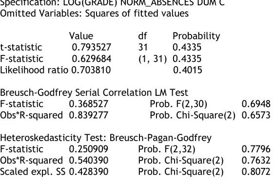
Ramsey RESET Misspecification Test

Specification: LOG(GRADE) NORM_ABSENCES DUM C Omitted Variables: Squares of fitted values

Value df Probability

t-statistic 0.793527 31 0.4335

F-statistic 0.629684 (1, 31) 0.4335

Likelihood ratio 0.703810 0.4015

Breusch-Godfrey Serial Correlation LM Test

F-statistic 0.368527 Prob. F(2,30) 0.6948

Obs*R-squared 0.839277 Prob. Chi-Square(2) 0.6573

Heteroskedasticity Test: Breusch-Pagan-Godfrey

F-statistic 0.250909 Prob. F(2,32) 0.7796

Obs*R-squared 0.540390 Prob. Chi-Square(2) 0.7632

Scaled expl. SS 0.428390 Prob. Chi-Square(2) 0.8072

Figure 4l: Structural Stability of the Parameters of the Model 2c: the Model is Stable.

4.40 4.44 4.48 4.52 4.56

2 3 24 25 26 2 7 2 8 29 30 31 3 2 33 34 35 R e cu rsi ve C(1) Es tim a te s

± 2 S.E.

-.020 -.015 -.010 -.005 .000 .005

2 3 24 25 26 2 7 2 8 29 30 31 3 2 33 34 35 R e cu rsi ve C(2) Es tim a te s

± 2 S.E.

-.16 -.12 -.08 -.04 .00

2 3 24 25 26 2 7 2 8 29 30 31 3 2 33 34 35 R e cu rsi ve C(3) Es tim a te s

± 2 S.E.

4 .4 0 4 .4 4 4 .4 8 4 .5 2 4 .5 6

23 24 25 26 27 28 29 30 31 32 33 34 35 Recurs ive C(1) Es tim ates

± 2 S.E.

-.0 2 0 -.0 1 5 -.0 1 0 -.0 0 5 .0 0 0 .0 0 5

23 24 25 26 27 28 29 30 31 32 33 34 35 Recurs ive C(2) Es tim ates

± 2 S.E.

-.1 6 -.1 2 -.0 8 -.0 4 .0 0

23 24 25 26 27 28 29 30 31 32 33 34 35 Recurs ive C(3) Es tim ates

± 2 S.E.

Figure 4m: Structural Stability of the Residuals of the Model 2c: the Model is Stable.

-12 -8 -4 0 4 8 12

20 21 22 23 24 25 26 27 28 29 30 31 32 33 34 35 CUSUM 5% Significance

-12 -8 -4 0 4 8 12

Figure 4n: Actual, Fitted Grades and Residuals: Normalized absences explain 32% of the total variation of the grades in the present model 2c. The remaining 68% of the variation cannot be explained by this model. -.2 -.1 .0 .1 .2 4.2 4.3 4.4 4.5 4.6

5 10 15 20 25 30 35 Residual Actual Fitted

-.2 -.1 .0 .1 .2 4.2 4.3 4.4 4.5 4.6

5 10 15 20 25 30 35 Residual Actual Fitted

Figure 4o: Static Forecast with 95% Confidence Interval. Figure 4p: Deterministic Simulation of

the Relation between Absences and

Absences and Grades.

60 70 80 90 100 110

5 10 15 20 25 30 35

GRA DE_FORECA ST ± 2 S.E.

Forecast: GRADE_FORECAST Actual: GRADE Forecast sample: 1 35 Included observations: 35 Root Mean Squared Error 5.487318 Mean Absolute Error 4.310534 Mean Abs. Percent Error 5.241986 Theil Inequality Coefficient 0.033024 Bias Proportion 0.001092 Variance Proportion 0.269073 Covariance Proportion 0.729835

60 70 80 90 100 110

5 10 15 20 25 30 35 GRADE_FORECAST ± 2 S.E.

Forecast: GRADE_FORECAST Actual: GRADE Forecast sample: 1 35 Included observations: 35 Root Mean Squared Error 5.487318 Mean Absolute Error 4.310534 Mean Abs. Percent Error 5.241986 Theil Inequality Coefficient 0.033024 Bias Proportion 0.001092 Variance Proportion 0.269073 Covariance Proportion 0.729835

65.00 70.00 75.00 80.00 85.00 90.00 95.00 0 .0 0 0 .9 0 1 .8 0 2 .7 0 3 .6 0 4 .5 0 5 .4 0 6 .3 0 7 .2 0 8 .1 0 9 .0 0 9 .9 0 1 0 .8 0 1 1 .7 0 1 2 .6 0 1 3 .5 0 1 4 .4 0 1 5 .3 0 1 6 .2 0 1 7 .1 0 1 8 .0 0 1 8 .9 0 1 9 .8 0

N orm alized Absences

G r a d e s

Exponential 2014 Exponential 2013 Linear 2014 Linear 2013

Figure 4q: Lag Selection Criteria: 1 lag is selected. Figure 4r: Stability of the VAR Process: All roots

are inside the unit circle. 1 time lag has been selected on the basis of all

lag order selection criteria.

-1.5 -1.0 -0.5 0.0 0.5 1.0 1.5

-1.5 -1.0 -0.5 0.0 0.5 1.0 1.5

Inverse Roots of AR Characteristic Polynomial

-1.5 -1.0 -0.5 0.0 0.5 1.0 1.5

-1.5 -1.0 -0.5 0.0 0.5 1.0 1.5

Figure 4s: Roots of Characteristic Polynomial.

Root Modulus

0.942682 0.942682

0.131343 0.131343

-0.085906 0.085906

No root lies outside the unit circle. VAR satisfies the stability condition

Figure 4t: Statistical Significance of the Lagged Parameters. None is significant.

Figure 4u: Impulse - Response Functions: Very Fast Monotonic Convergence to Zero.

-4 -2 0 2 4 6 8

1 2 3 4 5 6 7 8 9 10

Response of GR ADE to GR AD E

-4 -2 0 2 4 6 8

1 2 3 4 5 6 7 8 9 10

R esponse of GR AD E to N OR M _ABSEN C ES

-4 -2 0 2 4 6 8

1 2 3 4 5 6 7 8 9 10

Response of GRADE to DUM

-4 -2 0 2 4

1 2 3 4 5 6 7 8 9 10

R esponse of N OR M _ABSEN C ES to GR AD E

-4 -2 0 2 4

1 2 3 4 5 6 7 8 9 10

R esponse of N OR M _ABSEN C ES to N OR M _ABSEN C ES

-4 -2 0 2 4

1 2 3 4 5 6 7 8 9 10

Response of NOR M _ABSEN C ES to DU M

-.1 .0 .1 .2 .3

1 2 3 4 5 6 7 8 9 10

Response of DUM to GRADE

-.1 .0 .1 .2 .3

1 2 3 4 5 6 7 8 9 10

Response of DU M to NOR M _ABSENC ES

-.1 .0 .1 .2 .3

1 2 3 4 5 6 7 8 9 10

Response of DUM to DUM