Modeling and forecasting remittances in Bangladesh using the Box Jenkins ARIMA methodology

(1)

Munich Personal RePEc Archive

Modeling and forecasting remittances in

Bangladesh using the Box-Jenkins

ARIMA methodology

NYONI, THABANI

University of Zimbabwe, Department of Economics

26 February 2019

Online at

https://mpra.ub.uni-muenchen.de/92463/

(2)

Modeling and Forecasting Remittances in Bangladesh Using The Box-Jenkins ARIMA Methodology

Nyoni, Thabani

Department of Economics

University of Zimbabwe

Harare, Zimbabwe

Email: nyonithabani35@gmail.com

Abstract

This paper uses annual time series data on remittances into Bangladesh from 1976 to 2017, to model and forecast remittances using the Box – Jenkins ARIMA technique. Diagnostic tests indicate that REM is I (2). The study presents the ARIMA (2, 2, 0) model for predicting remittances in Bangladesh. The diagnostic tests further show that the presented parsimonious model is stable and acceptable for predicting remittances in Bangladesh. The results of the study apparently show that remittances inflows into Bangladesh are on a downwards trajectory. The paper suggests the need for strengthening Bangladesh’s emigration policy in order to improve remittances inflows into Bangladesh.

Key Words: Bangladesh, Forecasting, Remittances

JEL Codes: C53, F24

I. Introduction

Remittances as a building block of economic development in the developing countries continue to attract global attention in the recent time (Adebayo, 2013). Remittance is the better instrument to remove poverty (Martin, 1994; Murshid et al, 2001) and in fact, at present, remittances play a crucial role in the economy of Bangladesh (Hossain & Abdulla, 2017) and this has already been empirically confirmed by Siddique et al (2010) and Paul & Das (2011) amongst others. Between 1976 and 2010, a total of 6.8 million people emigrated temporarily from Bangladesh (BMET, 2010). Given restricted labor mobility across countries, Bangladesh’s emigration figure is quite significant. Revenues from remittances in the country exceed various types of foreign exchange inflow, particularly official development assistance and net earnings from exports. Remittance inflows to Bangladesh are increasing at an average annual rate of 19% in the last 30 years from 1979 to 2008 (Hussain & Naeem, 2009). Income from remittances has recently exceeded the 10-billion dollar mark, which has been 11.8% of the country’s Gross Domestic Product (GDP) in 2009 (BBS, 2010). At present, the remittance of Bangladesh is the largest source of foreign exchange earning of the country and apparently plays a critical role in alleviating the foreign exchange constraint and supporting the balance of payments, enabling imports of capital goods and raw materials for industrial development (Islam et al, 2018). The main purpose of this study is to model and predict remittances inflow in Bangladesh using ARIMA models.

(3)

In an African study, Adebayo (2013), examined remittances inflow into Nigeria using annual data from 1977 to 2009 and employed the ARIMA technique and revealed that remittances into Nigeria in the coming years will grow at an average of 6% per annum with its size as a percentage of GDP expected to reach about 11.4% by 2019. Hossain & Abdulla (2017) forecasted remittances of Bangladesh by ARIMA and Neural Network models and used data over the period 1987 to 2015 and established that the fluctuations of the forecasted series to original series by Neural Networks are less compared to ARIMA. In a recent study, Islam et al (2018) forecasted remittances of Bangladesh using ARIMA and GARCH models with data set ranging over the period January 1998 to December 2003 and found out that the ARIMA (0, 1, 1)(0, 2, 1)12 and the GARCH (2, 1) model appeared to be the best one.

III. Materials & Methods Box – Jenkins ARIMA Models

One of the methods that are commonly used for forecasting time series data is the Autoregressive Integrated Moving Average (ARIMA) (Box & Jenkins, 1976; Brocwell & Davis, 2002; Chatfield, 2004; Wei, 2006; Cryer & Chan, 2008). For the purpose of forecasting remittances in Bangladesh, ARIMA models were specified and estimated. If the sequence ∆dREMt satisfies an

ARMA (p, q) process; then the sequence of REMt also satisfies the ARIMA (p, d, q) process

such that:

∆𝑑_𝑅𝐸𝑀

𝑡 = ∑ 𝛽𝑖∆𝑑𝑅𝐸𝑀𝑡−𝑖+ 𝑝

𝑖=1

∑ 𝛼𝑖𝜇𝑡−𝑖 𝑞

𝑖=1

+ 𝜇𝑡… … … . … … … … . … … . [1]

which we can also re – write as:

∆𝑑_𝑅𝐸𝑀

𝑡= ∑ 𝛽𝑖∆𝑑𝐿𝑖𝑅𝐸𝑀𝑡 𝑝

𝑖=1

+ ∑ 𝛼𝑖𝐿𝑖𝜇𝑡 𝑞

𝑖=1

+ 𝜇𝑡… … … . . … … … . … … … [2]

where ∆ is the difference operator, vector β ϵⱤp

and ɑ ϵⱤq.

The Box – Jenkins Methodology

The first step towards model selection is to difference the series in order to achieve stationarity. Once this process is over, the researcher will then examine the correlogram in order to decide on the appropriate orders of the AR and MA components. It is important to highlight the fact that this procedure (of choosing the AR and MA components) is biased towards the use of personal judgement because there are no clear – cut rules on how to decide on the appropriate AR and MA components. Therefore, experience plays a pivotal role in this regard. The next step is the estimation of the tentative model, after which diagnostic testing shall follow. Diagnostic checking is usually done by generating the set of residuals and testing whether they satisfy the characteristics of a white noise process. If not, there would be need for model re – specification and repetition of the same process; this time from the second stage. The process may go on and on until an appropriate model is identified (Nyoni, 2018).

(4)

This study is based on a data set of annual remittances (REM) as a percentage of GDP into Bangladesh ranging over the period 1976 – 2017. All the data was taken from the World Bank.

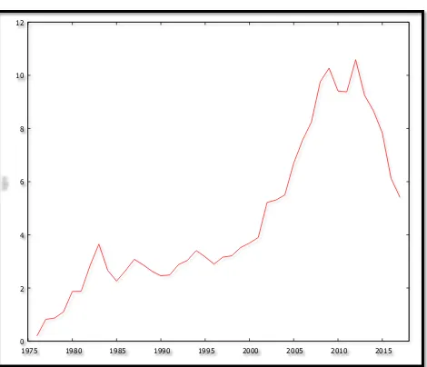
[image:4.612.81.551.173.577.2]

Diagnostic Tests & Model Evaluation Stationarity Tests: Graphical Analysis

Figure 1

The Correlogram in Levels

Autocorrelation function for REM ***, **, * indicate significance at the 1%, 5%, 10% levels.

Table 1

LAG ACF PACF Q-stat. [p-value]

1 0.9421 *** 0.9421 *** 40.0048 [0.000]

0 2 4 6 8 10 12

(5)

2 0.8713 *** -0.1448 75.0760 [0.000]

3 0.7916 *** -0.1062 104.7669 [0.000]

4 0.6901 *** -0.2299 127.9282 [0.000]

5 0.5901 *** -0.0111 145.3182 [0.000]

6 0.4865 *** -0.0835 157.4695 [0.000]

7 0.3885 ** 0.0174 165.4391 [0.000]

8 0.3030 ** 0.0287 170.4308 [0.000]

The ADF Test in Levels

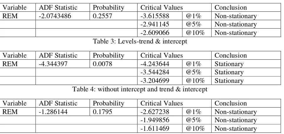
Table 2: Levels-intercept

Variable ADF Statistic Probability Critical Values Conclusion

REM -2.0743486 0.2557 -3.615588 @1% Non-stationary

-2.941145 @5% Non-stationary

[image:5.612.68.551.281.509.2]

-2.609066 @10% Non-stationary Table 3: Levels-trend & intercept

REM -4.344397 0.0078 -4.243644 @1% Stationary

-3.544284 @5% Stationary

Table 4: without intercept and trend & intercept

-1.611469 @10% Non-stationary As shown in figure 1 and tables 1 – 4, REM is non-stationary in levels.

The Correlogram (at 1st Differences)

Autocorrelation function for d_REM ***, **, * indicate significance at the 1%, 5%, 10% levels.

Table 5

1 0.3037 * 0.3037 * 4.0664 [0.044]

2 0.0490 -0.0477 4.1748 [0.124]

3 0.3496 ** 0.3848 ** 9.8442 [0.020]

(6)

5 -0.0528 0.0379 10.2221 [0.069]

6 0.1199 -0.0051 10.9465 [0.090]

7 -0.0857 -0.1424 11.3278 [0.125]

8 -0.3574 ** -0.3093 ** 18.1527 [0.020]

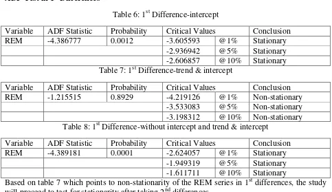
[image:6.612.65.548.177.456.2]

ADF Test in 1st Differences

Table 6: 1st Difference-intercept

REM -4.386777 0.0012 -3.605593 @1% Stationary

Table 7: 1st Difference-trend & intercept

-3.198312 @10% Non-stationary Table 8: 1st Difference-without intercept and trend & intercept

REM -4.389181 0.0001 -2.624057 @1% Stationary

Based on table 7 which points to non-stationarity of the REM series in 1st differences, the study will proceed to test for stationarity after taking 2nd differences.

The Correlogram (at 2nd Differences)

Autocorrelation function for d_d_REM ***, **, * indicate significance at the 1%, 5%, 10% levels.

Table 9

1 -0.3522 ** -0.3522 ** 5.3436 [0.021]

2 -0.3906 ** -0.5875 *** 12.0880 [0.002]

3 0.4273 *** 0.0035 20.3785 [0.000]

4 -0.1266 -0.2022 21.1260 [0.000]

5 -0.1584 -0.0761 22.3304 [0.000]

(7)

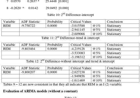
7 0.0570 0.2637 * 25.4448 [0.001]

8 -0.2620 * 0.0142 29.0492 [0.000]

Table 10: 2nd Difference-intercept

REM -9.758722 0.0000 -3.615588 @1% Stationary

Table 11: 2nd Difference-trend & intercept

REM -9.803464 0.0000 -4.219126 @1% Stationary

Table 12: 2nd Difference-without intercept and trend & intercept

REM -9.800207 0.0000 -2.627238 @1% Stationary

Tables 9 – 12 are now consistent in that they all indicate that REM is an I (2) variable.

[image:7.612.61.548.75.419.2]

Evaluation of ARIMA models (without a constant)

Table 13

Model AIC U ME MAE RMSE MAPE

ARIMA (1, 2, 1) 88.67342 0.83743 -0.099525 0.50405 0.67759 13.061 ARIMA (2, 2, 2) 84.03579 0.75728 -0.091833 0.46023 0.60568 11.989

ARIMA (3, 2, 0) 82.3836 0.78881 -0.082236 0.47481 0.61285 12.447

ARIMA (2, 2, 0) 80.98338 0.78638 -0.084635 0.47379 0.61321 12.383 ARIMA (1, 2, 0) 95.71541 0.98518 -0.054574 0.54986 0.76088 14.092 ARIMA (0, 2, 1) 86.67362 0.83764 -0.099554 0.50434 0.67758 13.07 ARIMA (2, 2, 1) 82.87394 0.79013 -0.079765 0.47479 0.61232 12.488 ARIMA (1, 2, 2) 86.87068 0.77317 -0.095322 0.46009 0.64532 11.74 A model with a lower AIC value is better than the one with a higher AIC value (Nyoni, 2018). Theil’s U must lie between 0 and 1, of which the closer it is to 0, the better the forecast method (Nyoni, 2018). The study will only consider the AIC as the criteria for choosing the best model for forecasting remittance inflows into Bangladesh and therefore, the ARIMA (2, 2, 0) model is carefully selected.

95% Confidence Ellipse & 95% 95% Marginal Intervals

(8)

Figure 2 indicates that the accuracy of the forecast given by the ARIMA (2, 2, 0) Model is satisfactory since it falls within the 95% confidence interval.

Stability Test

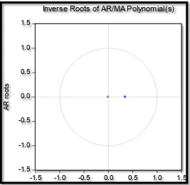
[image:8.612.78.550.75.294.2]

Stability Test of the ARIMA (2, 2, 0) Model

Figure 3

-1 -0.9 -0.8 -0.7 -0.6 -0.5 -0.4 -0.3 -0.2

-0.9 -0.8 -0.7 -0.6 -0.5 -0.4 -0.3 -0.2

-0.557, -0.586

phi_1

95% confidence ellipse and 95% marginal intervals

-1.5 -1.0 -0.5 0.0 0.5 1.0 1.5

A

R

r

o

ts

[image:8.612.172.439.423.683.2]

(9)

Since the corresponding inverse roots of the characteristic polynomial lie in the unit circle, it illustrates that the chosen ARIMA (2, 2, 0) model is stable and suitable for predicting remittances in Bangladesh over the period under study.

IV. Findings Descriptive Statistics

Table 14

Description Statistic

Mean 4.5814

Median 3.31

Minimum 0.19

Maximum 10.59

Standard deviation 2.9159

Skewness 0.69137

Excess kurtosis -0.75917

As shown above, the mean is positive, i.e. 4.5814%. The minimum is 0.19% and the maximum is 10.59%. The skewness is 0.69137 and the most striking characteristic is that it is positive, indicating that the REM series is positively skewed and non-symmetric. Excess kurtosis was found to be -0.75917; implying that the REM series is not normally distributed.

Results Presentation1

Table 15

ARIMA (2, 2, 0) Model:

∆𝑅𝐸𝑀𝑡−1= −0.556915∆𝑅𝐸𝑀𝑡−1− 0.586338∆𝑅𝐸𝑀𝑡−2… . . … … … . [3] P: (0.0000) (0.0000)

S. E: (0.1288) (0.1303)

Variable Coefficient Standard Error z p-value

AR (1) -0.556915 0.128839 -4.323 0.0000***

AR (2) -0.586338 0.130323 -4.499 0.0000***

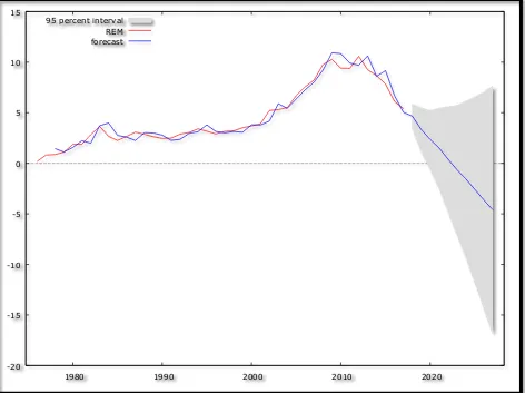
Forecast Graph

Figure 4

1

(10)

Predicted Annual Remittance Inflow into Bangladesh

Table 16

Year Prediction Std. Error 95% Confidence Interval

2018 4.66 0.610 3.46 - 5.86

2019 3.34 1.071 1.24 - 5.44

2020 2.36 1.454 -0.49 - 5.21

2021 1.52 2.003 -2.40 - 5.45

2022 0.41 2.632 -4.75 - 5.57

2023 -0.63 3.248 -7.00 - 5.73

2024 -1.55 3.929 -9.25 - 6.15

2025 -2.58 4.676 -11.75 - 6.58

-20 -15 -10 -5 0 5 10 15

1980 1990 2000 2010 2020

[image:10.612.79.551.77.430.2]

(11)

2026 -3.63 5.442 -14.29 - 7.04

2027 -4.60 6.246 -16.84 - 7.65

Figure 4 (with a forecast range from 2018 – 2027) and table 16, clearly show that remittance inflow into Bangladesh is currently on a downwards trajectory and is unfortunately projected to follow this path at least for the next decade, ceteris paribus. The most eye-catching feature of table 16 is that over the period 2023 – 2027, Bangladesh may receive no remittances inflows! This is shown by negative percentage contributions to GDP.

V. Conclusion & Policy Implications

The ARIMA model was employed to investigate annual remittances inflows into Bangladesh from 1976 to 2017. The study planned to forecast remittances for the upcoming period from 2018 to 2027 and the best fitting model was carefully identified. The ARIMA (2, 2, 0) model is stable and most suitable model to forecast remittances inflow into Bangladesh for the next ten years. From the study, it is inferred that Bangladesh as a leader among countries that receive remittances in Asia, may harness its potential adequately to significantly improve the livelihoods of Bangladeshi people. This means that the emigration policy must be strengthened to allow emigrants from Bangladesh (the leaving country) secure enough security and legality to facilitate the quality of the jobs they will engage in the host country, just because the size of their income is closely related to the size of fund to be expatriated to the home country (Bangladesh, in this case) in form of remittances.

References

[1] Adebayo, A (2013). Forecasting remittances as a major source of foreign income to Nigeria: evidence from ARIMA model, European Journal of Humanities and Social Sciences, 24 (1): 1255 – 1270.

[2] BBS (2010). Gross Domestic Product (GDP) of Bangladesh for 2004 – 2009, Bangladesh Bureau of Statistics (BBS).

[3] BMET (2010). Overseas employment and remittances from 1976 – 2010, Bureau of Manpower Employment and Training (BMET).

[4] Box, G. E. P & Jenkins, G. M (1976). Time Series Analysis: Forecasting and Control,

Holden Day, San Francisco.

[5] Brocwell, P. J & Davis, R. A (2002). Introduction to Time Series and Forecasting,

Springer, New York.

[6] Chatfield, C (2004). The Analysis of Time Series: An Introduction, 6th Edition, Chapman & Hall, New York.

(12)

[8] Hossain, M. M & Abdulla, F (2017). Forecasting remittances of Bangladesh by ARIMA and Neural Network Model, Conference Paper, Jahangirnagar University & Islamic University.

[9] Hussain, Z & Naeem, F (2009). Remittances in Bangladesh: Determinants and Outlook,

World Bank.

[10] Islam, T., Mohib, A. A., & Haque, S. Z (2018). Econometric models for forecasting remittances of Bangladesh, Business and Management Studies, 4 (1): 1 – 9.

[11] Martin, A. K (1994). The overseas migrant workers, remittances and the economy of Bangladesh: 1976/77 to 1992/93, Journal of Business Studies, 15: 87 – 109.

[12] Murshid, K. A. S., Iqbal, K., & Ahmed, M (2001). Migrant workers from Bangladesh Remittance inflows and utilization, Research Report.

[13] Nyoni, T (2018). Modeling and Forecasting Inflation in Kenya: Recent Insights from ARIMA and GARCH analysis, Dimorian Review, 5 (6): 16 – 40.

[14] Nyoni, T (2018). Modeling Forecasting Naira / USD Exchange Rate in Nigeria: a Box – Jenkins ARIMA approach, University of Munich Library – Munich Personal RePEc Archive (MPRA), Paper No. 88622.

[15] Nyoni, T. (2018). Box – Jenkins ARIMA Approach to Predicting net FDI inflows in Zimbabwe, Munich University Library – Munich Personal RePEc Archive (MPRA), Paper No. 87737.

[16] Paul, B. P & Das, A (2011). The remittance-GDP relationship in the liberalized regime of Bangladesh: cointegration and innovation accounting, Theoretical and Applied Economics, XVIII (9): 41 – 60.

[17] Siddique, A., Selvanathan, E. A., & Selvanathan, S (2010). Remittances and economic growth: empirical evidence from Bangladesh, India and Sri Lanka, Discussion Paper No. 10.27., The University of Western Australia.

[18] Wei, W. S (2006). Time Series Analysis: Univariate and Multivariate Methods, 2nd Edition, Pearson Education Inc, Canada.