Economic rationality under cognitive load

Munich Personal RePEc Archive

Economic rationality under cognitive

load

Drichoutis, Andreas C. and Nayga, Rodolfo

Agricultural University of Athens, University of Arkansas

20 August 2017

Online at

https://mpra.ub.uni-muenchen.de/88192/

Economic rationality under cognitive load

∗

Andreas C. Drichoutis

and Rodolfo M. Nayga, Jr.

1

Agricultural University of Athens

University of Arkansas

First Draft: August 20, 2017

This Version: July 25, 2018

Abstract: Economic analysis assumes that consumer behavior can be rationalized by a utility function. Previous research has shown that some consistency of choices with economic rationality can be captured by permanent cognitive ability but has not examined how a tempo-rary load in subjects’ working memory can affect economic rationality. In a controlled laboratory experiment, we exogenously vary cognitive load by asking subjects to memorize a number while they undertake an induced budget allocation task (Choi et al.,2007a,b). Using a number of ma-nipulation checks, we verify that cognitive load has adverse effects on subjects’ performance in reasoning tasks. However, we find no effect in any of the goodness-of-fit measures that measure consistency of subjects’ choices with the Generalized Axiom of Revealed Preference (GARP), despite having a sample size large enough to detect even small differences between treatments with 80% power. We also find no effect on first-order stochastic dominance and risk preferences. Our finding suggests that economic rationality can be attained even when subjects are placed under temporary working memory load and despite the fact that the load has adverse effects in reasoning tasks.

Keywords: Cognitive load, rationality, revealed preference, working memory, response times, laboratory experiment, risk

JEL codes: C91, D03, D11, D12, G11

∗_{We would like to thank Cary Deck and Salar Jahedi for sharing their zTree implementation of the cognitive}

load manipulation; Dan Burghart, Jan Heufer, Per Hjertstrand, Shachar Kariv, Daniel Martin and Bart Smeul-ders for sharing their data and codes; David Dickinson and Cary Deck for helpful comments and suggestions on an early draft of the manuscript; Dafni Koletti and Antigoni Patso for helpful research assistance. Approval for the research was provided by the Institutional Review Board of the University of Arkansas (#16-11-226) and the Board of Ethics and Deontology of the Department of Agricultural Economics & Rural Development at the Agricultural University of Athens (2/2016).

†_{Assistant Professor, Department of Agricultural Economics & Rural Development, Agricultural University}

of Athens, Iera Odos 75, 11855, Greece, e-mail: [email protected].

‡_{Distinguished Professor and Tyson Endowed Chair, Department of Agricultural Economics & Agribusiness,}

1

Introduction

Lately, there has been a lot of attention given to decision making ability as the driving force behind heterogeneity in choices. Choi et al. (2014) advance the view that the choices that some people make may be different from the choices they would make if they had the skills or knowledge to make better decisions. Thus, limited decision-making ability may produce sub-optimal choices indicative of low decision-making quality. The role of intelligence or cognitive ability has been the subject of many studies (see for example Bra˜nas Garza and Smith, 2016;

Rustichini,2015, and citations therein) and some of the stylized facts from this literature include the notion that people of high cognitive ability are more risk-tolerant, more patient, and less prone to anchoring effects than those with lower cognitive ability (see Deck and Jahedi, 2015, and citations therein).

The dual-system approach view in decision making offers a mechanism that can explain differences in decision making as a result of cognitive abilities. Under this approach, people have two distinct kinds of reasoning widely known as ‘System 1’ and ‘System 2’ (Stanovich and West, 2001). System 1 is considered the impulsive/intuitive system while system 2 is the reasoning system. The two systems differ in terms of working memory capacity, consciousness in reasoning, automaticity, speed etc. (Kahneman,2011). Given that working memory capacity is known to be highly correlated with reasoning ability (Kyllonen and Christal,1990), one direct implication of this fact is that System 2 functions should be related to measures of cognitive ability while System 1 functions should be independent of such measures.

In the dual-system approach, behavior is determined by the interaction of the two systems: System 1 will produce intuitive answers to problems as they arise while System 2, given enough time to engage, could override or correct automatic judgments. Therefore, by simply observing human behavior, it is hard to attribute decision making on either of the two systems. In order to disentangle the effects of the two systems, the economics literature has adopted a technique known as cognitive load manipulation, often used in the social psychology literature as well, that allows researchers to exogenously impair subjects’ cognitive resources. Following this line of research, our experimental treatment is designed to reduce availability of cognitive resources for concurrent tasks by requiring subjects to memorize numbers of different lengths while they are making choices. Imposing a burden on working memory has been shown to have adverse effects on performance in a variety of tasks that involve logic or reasoning (see Deck and Jahedi,2015, and citations therein). Deck and Jahedi (2015), based on an extensive review of the literature note that overall, increasing cognitive load leads to poorer reasoning and math performance, more risk-aversion, and more impatient choices.

over money, and a higher likelihood to anchor, but they find no evidence of cognitive load effects on impatience or unhealthy snack choice. Similarly,Benjamin et al. (2013) andGerhardt et al. (2016) find that a cognitive load manipulation increases risk aversion. Many other studies that are reviewed in Deck and Jahedi (2015) are exploring cognitive load in relation to math ability and logic, risk, intertemporal choice, food choice, generosity, strategic behavior etc.

By this account, our cognitive load manipulation (memorizing a number) is expected to load the reasoning system (‘System 2’). Hence, any decision that subjects perform when under cognitive load should be the outcome of ‘System 1’ which is the impulsive and intuitive system. Our research question is whether ‘System 1’ can produce decisions that can be characterized as of high decision-making quality in economic terms, or whether ‘System 2’ is necessary for subjects to make high quality decisions. FollowingChoi et al. (2014) we define decision-making quality in terms of whether observable behavior is consistent with the utility maximization model.

Using the utility maximization model as the benchmark by which to judge decision-making quality is quite natural for economic analysis and has strong theoretical and methodological justifications (Choi et al., 2014). Economic analysis assumes that consumer behavior can be rationalized by a utility function and this economic rationality assumption is by now well un-derstood and described by the core axioms of revealed preference theory (Afriat, 1967;Varian,

1982). Revealed preference theory also provides the tools to test whether any given data set violates those axioms and how severe such violations might be.

There are some scattered evidence in the literature linking economic rationality with mea-sures of cognitive ability which provide a rationale to examine the effect of a cognitive load manipulation on economic rationality. Choi et al. (2014) find a positive correlation of a mea-sure of consistency with economic rationality with the Cognitive Reflection Test (CRT) of

Frederick (2005) which is often considered a simple measure of cognitive ability. They also find that the CRT captures some decision-making ability related to decision-making quality in their experiment.

to choose budget allocations using the Choi et al. (2007a,b) allocation task.1

To establish the effectiveness of their manipulation, Castillo et al. (2017) first show that circadian matched and mismatched subjects do not differ in many measures (including self-reported sleep measures) before the experiment takes place. They then use the Karolinska sleepiness score to show that mismatched subjects report being significantly more sleep deprived than circadian matched subjects. Thus, they assume the existence of an adverse cognitive resource state due to sleep restriction, even though its effects are not directly tested in the experiment. Castillo et al.

(2017) find that adherence to the generalized axiom of revealed preference (GARP) is identical between mismatched and matched participants.

In our study, in order to explore consistency with economic rationality, we employ theChoi et al.(2007a,b) induced budget allocation task. This particular allocation task allows elicitation of many decisions per subject from a wide variety of budget lines. In addition, the shifts in income and relative prices are such that budget lines cross frequently and so the variety of budget lines produces data that can be used to test for consistency with revealed preference theory (Choi et al., 2007a). Our cognitive load manipulation, a number memorizing task, is designed along with several incentivized manipulation checks that undoubtedly show its effectiveness. We find that subjects’ performance in demanding reasoning tasks is affected when under high cognitive load but less so in tasks that require low or no reasoning at all. We employ several goodness-of-fit measures to measure consistency with economic rationality given the trade-offs involved with using one over another, and generally find that cognitive load does not affect economic rationality; i.e., a null effect. We also show that our study was sufficiently powered to detect even small effects, which gives us enough confidence to conclude that our null effect is genuine and not the result of a small sample size. We also report a null effect with respect to first-order stochastic dominance and risk preferences.

The next section describes our experimental design with particular emphasis on the cognitive load manipulation and the induced budget line allocation task. Section 3 describes the various goodness-of-fit measures we use in this study to measure consistency with economic rationality according to revealed preference theory. In Section 4 we showcase the null effect of cognitive load on economic rationality after first establishing the success of the treatment based on a series of manipulation checks. We also complement our results with sample size calculations to show that our null result is likely not a false negative.

1

2

Experimental design

In May 2017, we recruited 178 subjects from the undergraduate population of the Agri-cultural University of Athens in Greece to participate in a computerized experiment at the Laboratory of Behavioral and Experimental Economics Science (LaBEES-Athens). Subjects were recruited using ORSEE (Greiner, 2015) and participated in 10 sessions of 14 to 25 sub-jects. All sessions started at 10 am and concluded by 2 pm. Although subjects participated in group sessions, there was no interaction at any point between subjects and group sessions only served as a means to economize on resources. In fact, given that we timed every decision stage of our experiment (response times are discussed in Section 2.4), we chose to run individ-ual instances of zTree (Fischbacher, 2007) to avoid any time lags in communication between computers and allow every participant to proceed at their own pace. Although subjects knew from the very beginning that they could move through the screens at their own pace, they were also told that they could leave the room only when all the subjects have made their decisions for reasons related to collection of all data and the printing of the individual receipts. This was also done to slow down the pace of subjects who just wanted to minimize their stay in the lab.2

Subjects were randomly split into two between-subjects treatments and each subject was only exposed to one of them: 87 subjects experienced the high cognitive load treatment (HCL) and 91 subjects experienced the low cognitive load (LCL) treatment.

Upon arrival, subjects were given a consent form to sign and were randomly seated to one of the PC private booths. The instructions were computerized, interactive and included thorough examples for each type of task that would appear in the experiment (see Experimental Instruc-tions section in the Electronic Supplementary Material). Subjects were specifically instructed to raise their hand and ask any questions in private and that the experimenter (one of the authors) would then share his answer with the group. Subjects received a show-up fee of e_{3 and a fee}

of e_{4 for completing the experiment so that each subject would receive}e_{7 with certainty upon}

successful completion of the experiment, which lasted about an hour. They could also earn additional money during the experiment (described momentarily), and so the average of total payouts was e_{13.05 (S.D.=3.64, min=7, max=20.53).}

In total, subjects played 75 periods and in every period they went through one of the following decision tasks: 1) an induced budget line allocation task, 2) an arithmetic (addition) task, 3) an arithmetic (multiplication) task, and 4) a click-a-button task. The budget allocation task was repeated for 60 consecutive periods (reasons for this number of repetitions are explained in Section 2.2) and every other decision task was repeated for 5 consecutive periods (thus, 1 task

× 60 periods + 3 tasks × 5 periods = 75 periods). Subjects were not provided with any kind

2

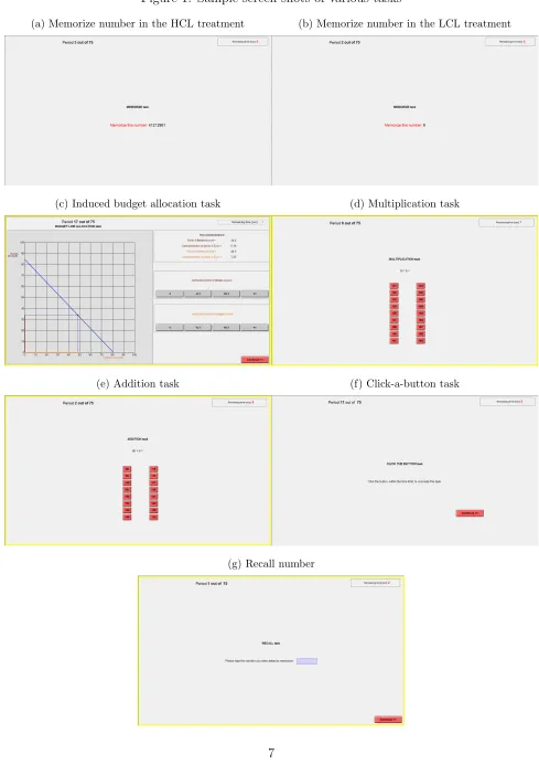
of feedback between periods for any of the tasks. Each subject was randomly exposed to one of the possible orders of the tasks; however, the induced budget task was always placed either at the very beginning of the experiment or at the very end. Figure 1 shows sample screen shots illustrating the various decision tasks.

Subjects were specifically instructed to remove from their desks anything that could be used to take notes (e.g., cellphones, paper, pen, pencil etc.). This was part of their instructions (see Experimental Instructions - Screen 1 at the Electronic Supplementary Material) but they were also reminded orally by the experimenter before the start of the experiment. In addition, two research assistants and the experimenter supervised the lab to make sure that this would be enforced during the experiment so that subjects could not cheat in any way at the memorization task by, for example, typing the number they had to memorize in an intermediate screen. This also affected the way we designed all other tasks in that we avoided having input boxes (which subjects could use to temporarily type the number they had to memorize) and only included buttons as input items. Shortcut keys for copy-paste (i.e., ctrl+c and ctrl+v) were disabled in all computers during the experiment.

2.1

Cognitive load manipulation

To manipulate cognitive load, we implemented an incentivized number memorization task (Benjamin et al.,2013;Deck and Jahedi,2015).3

Specifically, in each period and just before the main decision tasks described above, a number appeared for four seconds on the participant’s computer screen (see Figure 1a and 1b for sample screen shots). Subjects were then asked to keep this number in their memory and recall it after the main decision task (see Figure 1g for a sample screen shot). If they recalled (typed) the number correctly within a time limit of ten seconds, their memorization payoff for the period wase_9.4

Otherwise it wase_{0. Subjects in the}

HCL treatment were shown 8-digit numbers while subjects in the LCL treatment were shown 1-digit numbers to memorize. Numbers to memorize where drawn randomly in each period and independently from other subjects.

3

Benjamin et al. (2013) note that requiring participants to memorize a string of numbers while they are engaged in the task of interest is a common cognitive load manipulation in the psychology literature (e.g., Hinson et al.,2003;Shiv and Fedorikhin,1999). Furthermore, Deck et al.(2017) experimentally test the effects of four commonly used techniques for manipulating cognitive capacity, namely a number memorization task, a visual pattern task, an auditory recall task, and time pressure. They find that the number memorization and auditory recall tasks are the most reliable techniques for inducing cognitive load among those considered in their study.

4

Figure 1: Sample screen shots of various tasks

(a) Memorize number in the HCL treatment (b) Memorize number in the LCL treatment

(c) Induced budget allocation task (d) Multiplication task

(e) Addition task (f) Click-a-button task

2.2

The induced budget line allocation task

We used the graphical representation of simple allocation choice tasks ofChoi et al.(2007b) where subjects are asked to select a bundle of commodities from a standard budget set. Subjects saw a graphical representation of a budget line on the computer screen and made choices on the budget line through a simple point-and-click action (see Figure 1c). In our implementation of the interface in zTree, we also allowed subjects to make refined grid choices by using buttons that could add/subtract very small amounts in the commodity space in an interactive way.

This particular interface allows elicitation of many decisions per subject from a wide variety of budget lines which produces a very rich individual-level dataset. The shifts in income and relative prices are such that budget lines cross frequently and the variety of budget lines produces data that have been used in the literature to test if the Generalized Axiom of Revealed Preference (GARP) holds (Choi et al., 2007a). If GARP holds, then an individual’s choices are consistent with maximization of a well-behaved utility function.5

Choi et al.(2014) use this consistency of choices with economic rationality as a measure of decision-making quality (economic rationality defined by having a complete and transitive preference ordering).

In the induced budget line allocation task, subjects were asked to choose an allocation of points (constrained to lie on the budget line) between the ‘Orange account’ and the ‘Brown account’ (corresponding to the horizontal and vertical axis, respectively) with the understanding that one of the accounts would be randomly selected at the end of the experiment and that each account was equally likely. Each task started with the computer selecting a budget line randomly from the set of budget lines that intersect with at least one of the axis at 50 or more points and the other axis at 30 or more points. No intercept could exceed 100 points. The budget lines selected were independent between periods and between subjects (the full set of budget lines shown to each subject and their respective choices can be found in the Electronic Supplementary Material). The pointer was set by default to the origin, if subject had not yet made a choice. Although a timer was implemented for consistency with the other tasks, subjects were not forced out of the task if they had not made a choice. The exchange rate between points and Euros was set to 1 point = e_0.15.

The number of periods in the induced budget line allocation task was determined based on

Bronars’s (1987) power measure of revealed preference tests. Bronars (1987) adopted Becker’s (1962) notion of irrational behavior where the representative consumer is assumed to choose

5

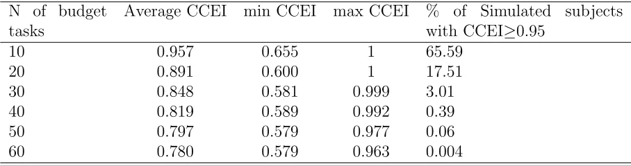
consumption bundles randomly from her budget hyperplane. We randomly generated consump-tion data for 50,000 hypothetical subjects who randomize uniformly among all allocaconsump-tions on each budget line and repeated this procedure over 10 to 60 budgets tasks with a step of 10. We then calculated Afriat’s Critical Cost Efficiency index (CCEI) which measures the amount by which each budget constraint must be relaxed in order to remove all violations of GARP (Afriat, 1972; Varian, 1993, 1990) (see also section 3.1 for a detailed description of this index).

Varian(1993) proposes a 95% efficiency level as the critical level for “sentimental reasons [sic]”. Table 1 shows that increasing the number of budget tasks from 10 to 60 significantly reduces the chance that random behavior will pass the GARP test. With 60 budget tasks, only 2 out of 50,000 hypothetical subjects have a CCEI larger than 0.95. The number of repetitions is an important detail in our design because under cognitive load, there might be a tendency for subjects towards random choice. Therefore, we wanted to make sure that by design, there is a very low chance of random behavior passing as consistent with GARP. Given the trade-off involved with adversely affecting the duration of any given session when increasing the number of periods, we opted to repeat the induced budget allocation task for 60 periods.

Table 1: Number of budget tasks and Afriat’s Critical Cost Efficiency index (CCEI) for randomly generated consumption data for 50,000 simulated subjects

N of budget tasks

Average CCEI min CCEI max CCEI % of Simulated subjects with CCEI≥0.95

10 0.957 0.655 1 65.59

20 0.891 0.600 1 17.51

30 0.848 0.581 0.999 3.01 40 0.819 0.589 0.992 0.39 50 0.797 0.579 0.977 0.06 60 0.780 0.579 0.963 0.004

2.3

Arithmetic and click-a-button tasks

The arithmetic and click-a-button tasks were used as manipulation checks in order to identify whether the number memorization task actually manipulates cognitive load. The tasks were meant to differ in terms of task difficulty in order to assess the severity of the manipulation on decision making.

In the multiplication arithmetic task, subjects had to multiply a one-digit integer m1 ∼

U{5, . . . ,9} and a two-digit integer m2 ∼ U{13, . . . ,19}. In the addition arithmetic task,

sub-jects had to add a one-digit integera1 ∼U{1, . . . ,9}and a two-digit integera2 ∼U{11, . . . ,99}.6

6

Subjects had to indicate their answer by clicking the right choice from a list of randomly deter-mined 16 possible choices that were shown in two columns in an ordered manner; i.e., from low values to high values (see Figures 1d and 1e). The correct answer was set randomly to one of the buttons.

In the a-button task, subjects simply had to click a button. The arithmetic and click-a-button tasks were set with a time limit of 11 seconds after which subjects would be forced out if they had not made a decision.7

If subjects performed any of the tasks described above correctly, their payoff for the period was e_{7. Otherwise it was zero.}

The tasks varied in terms of difficulty in the following manner: multiplication ≫ addition

≫ click-a-button. Our intention with this manipulation check was to see whether memorizing a large number affects ability to perform difficult tasks (like multiplication and addition) but not ability to perform simple tasks (like clicking a button). We would expect that performance in the multiplication task, a much harder task than addition, would be more adversely affected under cognitive load.

2.4

Response times

Although interest around response times (RT) and their relevance for economic analysis has been increasing lately (see for example discussions in Clithero,2018;Spiliopoulos and Ortmann,

2018), response times have not been recorded and analyzed in previous studies that involved cognitive load manipulations (e.g., Benjamin et al., 2013; Deck and Jahedi, 2015). However, RT have been given prompt attention in more recent studies (Gerhardt et al., 2016).

Response times are particularly useful if one adopts the dual-system approach view in de-cision making (Stanovich and West, 2001). Since the two systems differ in terms of working memory capacity, consciousness in reasoning, automaticity, speed etc., response times could serve as an indicator of which system is dominating as well as an indicator of the difficulty of a task (Gerhardt et al., 2016).

Given that the cognitive load manipulation (memorizing a number) is expected to load the reasoning system (‘System 2’), any decision that the subjects perform when under cognitive load should be the outcome of ‘System 1’. If subjects really need to use ‘System 2’ to make a reasoning type decision, then they would need to really try hard to engage this system, which would be reflected in their response time. That said, we should be cautious when interpreting results from RT data in our paper because the treatment used in our study (having to type a long vs a short number) is naturally related to decision times. Furthermore, it is possible that response times could only be a remote proxy of what subjects would actually think when making decisions. For example, subjects may take longer time to decide because they could

7

be worried that making faster decisions would induce them to forget the number they were supposed to memorize. Similarly, taking more time to recall and report a number may pose little harm in terms of forgetting the number from not rushing and avoiding mistakes. All in all, while decision times may contribute in supporting intuitive explanations of the results, they should always be taken with a grain of salt.

To achieve a high precision in recorded times, each computer run an individual session of zTree/zLeaf for each subject, which factored out any latency due to network/computer commu-nication.

2.5

Measured cognitive ability

The cognitive load manipulation allowed us to vary the working-memory (WM) load of subjects while they completed other decision tasks. Working memory capacity has been shown to be strongly correlated with general cognitive ability (Colom et al., 2004; Gray et al., 2003). Therefore, before we apply the cognitive load manipulation, we first measured the cognitive ability of all subjects using the Raven’s Standard Progressive Matrices (RSPM) test which is used to assess mental ability associated with abstract reasoning and is considered a nonverbal estimate of fluid intelligence (Gray and Thompson,2004). The original RSPM test consists of 60 items and requires considerable time to complete. In this study, we used an abbreviated 9-item form of the RSPM test (Bilker et al.,2012) consisting of items 10, 16, 21, 30, 34, 44, 50, 52, 57 from the original 60-item Raven’s test. Subjects were not provided with any feedback regarding their performance in the RSPM test. The RSPM test allows us to sum correct responses and form a measure of cognitive ability that we can use to assess the effect of WM capacity on behavioral tasks’ performance.

2.6

Payoffs and payments

Participants were paid for one randomly drawn period (out of 75 periods) and for only one of the (randomly determined) tasks of this randomly selected period (i.e., either the memorization task or the decision task; depending on the period that was randomly drawn, the decision task could be either the induced budget line task or the addition task or the multiplication task or the click-a-button task). This was clearly explained beforehand in the instructions (see Experimental Instructions - Screen 2 in the Electronic Supplementary Material).

Similar to Deck and Jahedi (2015), we set the payoff associated with memorization (e₉₎

higher than the payoff for the multiplication task (e_{7), the addition task (}e_{7) and the}

click-a-button task (e_{7), so that participants (even the ones with limited working memory capacity)}

not involve certain payoffs, we calculated the expected payoff for the maximum induced budget line (i.e., cutting both axes at 100 points) and then calculated the expected payoff for a subject that either allocates everything to one account or splits points between the two accounts. Given an exchange rate of 1 point =e_{0.15, this expected payoff amounts to}e_{7.50, which is very close}

to the payoff of the other decision tasks.

Subjects received feedback about the randomly selected period and task only after they made all their decisions. Monetary payouts were paid via bank transfer to subject’s preferred bank account.8

3

Goodness-of-fit measures for rationality

We measure economic rationality in terms of whether our experimentally generated data can be rationalized by a utility function. We know by revealed preference theory (Afriat, 1967;

Varian, 1982) that individual’s choices can be rationalized by a utility function, if and only if the data satisfy the Generalized Axiom of Revealed Preference (GARP). GARP posits that if allocationxi is revealed preferred toxj, thenxj is not strictly directly revealed preferred toxi

or that if pixi ≥pixj then it cannot be that pjxj >pjxi (Varian,1982, p. 947).

The problem with empirically testing GARP is that the test is exact; i.e., data can either satisfy GARP or not. The test allows no errors in measurement or choice so that a single choice is enough to render a large choice set incompatible with rationality. Instead, goodness-of-fit (GOF) measures or indexes allow us to quantify the extent of such violations. Some of the more recently developed indexes have been constructed in order to address shortcomings of previously developed GOF measures. We briefly summarize some of these measures (starting from older measures and moving to more recently developed ones) and describe how we went about it with our data.

3.1

Afriat’s Critical Cost Efficiency index (CCEI)

Afriat’s Critical Cost Efficiency index (CCEI) measures the amount by which each budget constraint (such as the solid lines in Figure 2) must be relaxed (i.e., shifted to the dashed lines in Figure 2) in order to remove all violations of GARP (Afriat, 1972;Varian, 1993,1990). More formally, for 0 ≤ e ≤ 1 define the directly revealed preference relation xjRd(e)xi ⇔ epjxj ≥ pjxi. We can relax the directly revealed preference relation by defining the transitive

8

closure of Rd(e) as R(e). Afriat’s CCEI, e∗_{, is the largest value of e such that the relation R(e)}

satisfies GARP. In Andreoni et al. (2013) this version ofVarian’s (1993) GARP is refered to as L-GARP(e) (where ‘L’ is for ‘Lower’) and is defined as: xjR(e)xk ⇔epkxk ≤pkxj for e ≤1.

Ife∗ _{= 1, there is no violation of GARP while the larger the deviation from 1, the more a set of}

data fails to satisfy GARP. Researchers often follow Varian’s (1993) suggestion to use the 95% efficiency level as the critical level.

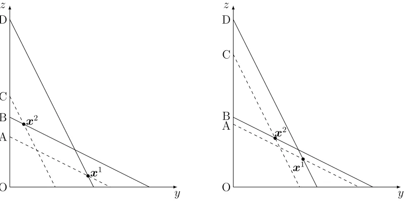
To illustrate the formulation of Afriat’s CCEI, consider Figure 2 where a simple revealed preference violation is depicted for the bundles x1 and x2. Bundle x1 is chosen at prices p1

when x2 is feasible so that we can infer that x1Rdx2. In addition, bundle x2 is chosen at prices p2 when x1 is feasible so that we can infer that x2Rdx1. Therefore, the choices depicted in

Figure2violate revealed preference axioms. The left figure depicts a more severe violation than the right figure. We can remove this violation by moving the budget line from B to A or from D to C. Afriat’s CCEI is related to the smallest shift we have to make to remove the violation, so in this case CCEI will be equal to OA/OB. Note that OA/OB will be closer to 1 in the right figure than in the left figure which indicates a less severe violation.

Technically, Afriat’s CCEI requires the computation of the transitive closure and there have been two approaches used in the literature for this. One of the approaches uses Warshall’s (1962) algorithm as described inVarian(1982,1996). The other approach computes the matrix power of the direct revealed preference matrix (also described in Varian, 1996). In this paper, we used both approaches and find that the computed CCEI is largely the same with the use of either method (the correlation coefficient between the two indexes is 0.97).9

9

Figure 2: A simple revealed preference violation y z O D x2 C B x1 A y z O D x2 C B x1 A

Notes: Bundle x1 is directly revealed preferred to bundle x2 and vice versa. The left graph

indicates a more severe violation than the right graph.

3.2

The Houtman—Maks Index (HMI)

TheHoutman and Maks(1985) index follows a different approach and measures the maximal number of observations in the observed sample consistent with rational choice. An advantage is that, if desired, the researcher can restrict the analysis to choices that are consistent with economic rationality.

Older attempts to calculate the HMI have cited computational intensity as the biggest drawback of the method (e.g., Choi et al., 2007a). More recently, Heufer and Hjertstrand

(2015) introduced simple and efficient algorithms for computing the HMI: Gross and Kaiser’s (1996) combinatorial algorithm and an algorithm based on solving a mixed-integer programming problem. As noted in Gross and Kaiser (1996), their algorithm sometimes fails to provide a maximal subset and only provides a lower bound. We confirm that this is sometimes the case with our data and so we based the HMI calculation on solving the mixed-integer programming problem as set up in Heufer and Hjertstrand (2015).10

3.3

The Money Pump Index (MPI)

A drawback of the HMI is that the method flags observations that violate revealed preference, even if they only violate it by a small amount. An alternative is the MPI which measures the severity of a violation in terms of a money metric (Echenique et al.,2011). This measure received

10

its name from the idea that a consumer who violates GARP could be potentially exploited as a ‘money pump’. This is because an arbitrager that knows the choices of a subject that violates GARP could follow the opposite purchasing strategy and resell the goods to the subject at a profit. Therefore, MPI is the amount of money that could be extracted from the consumer, expressed as a percentage of expenditure.

To illustrate the MPI, consider Figure 2 depicting a revealed preference violation. Assume a subject buys bundle x1 at prices p1 and bundle x2 at prices p2. An arbitrager would buy

bundle x1 at prices p2 and bundle x2 at prices p1 and then resell bundle x1 at prices p1

and bundle x2 at prices p2 to the subject. The arbitrager would then make a profit mp = x1(p1−p2) +x2(p2−p1) = p1(x1−x2) +p2(x2−x1). The left graph in Figure 2 depicts a

higher money pump cost than the right figure (mplef t > mpright), rendering the violation more

severe.

A practical difficulty in the computation of the MPI is that given multiple violations of revealed preference, there will be a money pump cost associated with each violation. To sum-marize multiple money pump costs in a single metric,Echenique et al.(2011) proposed the use of the mean and median money pump costs as an aggregate MPI. Given the computational burden involved in computing these aggregate money pump costs, Echenique et al. (2011) suggested to instead compute approximations of the mean and median MPIs. However, these approxi-mations focus on violations of revealed preference axioms that involve only a small number of observations (in Echenique et al. (2011) they report mean/median MPI for cyclic sequences of allocations of length up to 4).

Smeulders et al.(2013) proposed to measure the maximum and minimum MPIs for the most severe and the least severe violations, respectively, as easy-to-apply alternatives. The advantage is that max and min MPIs can be computed efficiently even for large datasets (i.e., defined over all violations). In this paper, we use the Smeulders et al. (2013) approach and calculated the min/max MPI for all possible violations.

3.4

The Minimum Cost Index (MCI)

data set (the sum of all relations) or by each subject’s total budget. We use both normalizations in our paper.

4

Results

Before we analyze our data for the estimation of treatment effects, we will first try to establish whether the effect from our experiment can be interpreted as causal. Typically, experimentalists use statistical tests (often called balance tests) to test for equality of various covariates between treatments. A failure to reject the null is interpreted as a good balance of observable character-istics between treatments and a success of the randomization process. Briz et al. (2017) provide a discussion over the literature that points to the pitfalls of statistical tests, often called balance tests, to test for differences between observable characteristics (e.g., Deaton and Cartwright,

2016; Ho et al., 2007; Moher et al., 2010; Mutz and Pemantle, 2015). Following Deaton and Cartwright’s (2016) advice, we report instead the normalized difference in means (Imbens and Rubin, 2016; Imbens and Wooldridge, 2009).

Table2 reports the descriptive statistics for a few observable characteristics of our subjects. As evident, the means are very close between the two groups while the median values are identical. Table 2 also reports a normalized difference measure |x¯1−x¯2|/

p

(s2 1 +s

2

2)/2 where

¯

xj and s2j (j = 1,2) are the group means and variances, respectively. The normalized difference

measure is a scale-free measure of differences in means scaled by the square root of the average of the two group variances. Cochran and Rubin’s (1973) rule of thumb is that the normalized difference should be less than 0.25 and Imbens and Rubin (2016) devote a full chapter to show that regression methods tend to be sensitive to the specification when normalized differences are large. As evident, the observable characteristics in our data pass this rule of thumb.

Table 2: Means of observable characteristics per treatment

HCL LCL Normalized difference Gender: Males 34.48% 31.87% 0.055

Household size 4.11 (1.04) [4] 4.30 (1.06) [4] 0.020 Age 21.33 (1.17) [21] 21.31 (1.35) [21] 0.173 Reference income 3.98 (1.49) [4] 4.23 (1.47) [4] 0.198 Raven test score 7.61 (1.43) [8] 7.32 (1.50) [8] 0.117 Raven test past experience 27.59% 32.97% 0.171

4.1

Difficulty of the memorization task

We now turn into exploring if the variation in the difficulty of the memorization task was significantly different between treatments. The top panel in Table 3 shows the frequency of correctly recalling the number in the memorization task (success rate) at the end of each period by treatment. The table shows the success rate after each task and when combined over all tasks. When comparing between treatments, it is obvious that the success rate in the HCL treatment was significantly lower. In fact, a χ2

test rejects the null for all rows in the top panel of Table 3(p-value<0.001) indicating that memorizing and correctly recalling an 8-digit number was significantly more difficult than memorizing and correctly recalling a 1-digit number. However, the difficulty of recalling the number varied depending on the intermediate task that was performed. For example, correct recall was as low as 8.97% after the multiplication task and was as high as 36.72% after the induced budget line task in the HCL treatment. Success rates improved for the addition task and further improved for the click-a-button task, suggesting the progressive difficulty of the tasks as we move from the click-a-button task to the addition task and then to the multiplication task. A χ2

test indicates that differences in success rate between tasks are statistically significant as well (p-value <0.001) for both the HCL and LCL treatments.

The second panel in Table 3 breaks down the percentage of successful recalls based on the count of numbers people correctly typed (for example, if a subject was required to memorize ‘37082109’ but then typed ‘69082109’, then this subject would have correctly typed six out of eight numbers). This might be important because a high count of correctly typed numbers is an indication that subjects put effort in the recall task, even though they did not get the entire set of numbers correctly. Table 3 shows that 72.51% of the times subjects correctly recalled 4 or more digits while 11.49% of the times subjects typed 3 digits or less correctly. Only, 16% of the times did subjects not submit a number at all. Overall, this is an indication that subjects treated the recall task seriously and did not give up because of the difficulty of the task.

The third panel in Table 3 shows how long it took subjects to recall (type in) the number they had memorized, irrespective of whether they gave a correct answer or not. Recorded times reflect the difficulty of the number memorization task. It took around 7 seconds to type and submit an answer in the HCL treatment and only about 2.3 secs in the LCL treatment. All differences are statistically significant between treatments according to Kruskal-Wallis tests (p-value<0.001). There is also significant variation between tasks. It took significantly longer for subjects to recall the number after the multiplication task than after the induced budget line task. Response times between tasks are also statistically significantly different according to Kruskal-Wallis tests for both the HCL and LCL treatments (p-value<0.001).

Table 3: Success rate and mean [median] decision time (in secs) in the recall task

HCL LCL

Success rate

Combined over all tasks 33.64% 97.67%

After. . .

Budget line 36.72% 98.37% Multiplication 8.97% 89.23% Addition 20.69% 96.92% Click-a-button 34.25% 98.46%

Success rate

All 8 digits 33.64% -7 digits 8.89% -6 digits 11.42% -5 digits 10.19% -4 digits 8.37% -3 digits or less 11.49% -Did not submit

a number 16.00%

-Decision time

Combined over all tasks 7.07 [6.80] 2.31 [2.17]

After . . .

Budget line 6.96 [6.64] 2.16 [2.06] Multiplication 7.71 [7.81] 3.15 [2.84] Addition 7.68 [7.55] 2.87 [2.62] Click-a-button 7.21 [7.03] 2.67 [2.44]

Decision time for correct recall

Combined over all tasks 6.21 [6.06] 2.26 [2.17]

After . . .

Budget line 6.18 [6.03] 2.13 [2.05] Multiplication 6.95 [6.72] 2.98 [2.76] Addition 6.72 [6.58] 2.81 [2.61] Click-a-button 6.17 [6.00] 2.61 [2.43]

Notes: HCL (LCL) stands for the high (low) cognitive load treatment. Differences between treatments (HCL vs. LCL) are statistically significant (p-value<0.001) for all rows of the table based on a χ2

test (for the top panel) and a Kruskal-Wallis test (for the medium and bottom panels). Differences between tasks are statistically significant (p-value<0.001) based on aχ2

subjects that correctly recalled the number. The picture is similar to what was discussed above, with response times reflecting the difficulty of the tasks in the sense that subjects spent a longer time to recall the number after a task that was intended to be more difficult. One interesting observation when we compare the bottom panel to the penultimate panel is that when subjects in the HCL treatment correctly recalled the number, it took them less time to do so, suggesting that spending more time trying to recall the number signified being less certain about the correct answer. In contrast, the differences are not significant under the LCL treatment when we compare the medium and bottom panels. This is probably because most of the subjects were able to correctly recall the 1-digit number most of the time.11

Next, in order to explore the differences in the success rate and recall time after the various decision tasks while taking into account control variables, we estimate various econometric models. Given the binary nature of the success/failure to recall the number, we estimate a logit model for the success/failure of recalling the memorized number. To condition response times on a set of independent variables, we have to consider that subjects’ responses were censored from above due to the time limit of the recall task, so we estimate a censored regression model with an upper limit of 10. All models are estimated with clustered standard errors to take into account the multiple responses given by the same subject and to allow for correlation between responses; i.e., it relaxes the independence assumption and requires only that the observations be independent across the clusters.12

Table 4 exhibits the results from a logit regression where success/failure is the dependent variable (model (1)) and results from two censored regression models where response time is the dependent variable. In model (2), we consider response times irrespective of whether subjects correctly recalled the number, while in model (3) we restrict the model to the subsample of response times with a correct recall of the number. All regressions control for the set of observable characteristics shown in Table 2. We also tried fitting models with interaction terms between the treatment variable and the task dummies but none of the interaction effects were statistically significant.

Results in Table 4 largely confirm our discussion above. The HCL treatment leads to a statistically significant lower success rate in correctly recalling the number. The difficulty of the 8-digit memorizing task is also reflected in the fact that subjects take more time to type

11

As a side note, one could attribute the differences in terms of decision time between the HCL and LCL treatments to the mechanics of the task i.e., the fact that given the mechanical nature of typing a number, it takes more time to type an 8-digit number rather than a 1-digit number. However, typing the number cannot be the sole explanation of the differences we observe in decision times between the two treatments. This is because the difference of the median decision times (combined over all tasks) in the medium panel of Table3is (roughly) 4.6 secs while for the bottom panel of the same table, it is (roughly) 3.9 secs. Thus, a difference of at least 0.7 secs should be attributed to differences in decision or response styles and not solely on the mechanics of the recall task.

12

Table 4: Logit regression of recall success/failure and Censored regressions of recall time

Recall success Recall time

. . . overall . . . for correct recall

(1) (2) (3)

Constant 1.878 (1.942) 5.741∗∗∗ _{(1.379) 5.578}∗∗∗ _(0.918)

Task: Budget line 1.656∗∗∗ _{(0.166) -0.562}∗∗∗ _{(0.102) -0.499}∗∗∗ _(0.083)

Task: Addition 1.119∗∗∗ _{(0.194) -0.178}∗∗ _{(0.082) -0.194}∗∗∗ _(0.074)

Task: Click-a-button 1.804∗∗∗ _{(0.172) -0.533}∗∗∗ _{(0.094) -0.482}∗∗∗ _(0.087)

HCL treatment -4.692∗∗∗ _{(0.168) 4.864}∗∗∗ _{(0.147) 4.044}∗∗∗ _(0.109)

Period 0.009∗∗∗ _{(0.002) -0.013}∗∗∗ _{(0.001) -0.012}∗∗∗ _(0.001)

Demographics Yes Yes Yes

σu - - 1.640∗∗∗ (0.063) 1.100∗∗∗ (0.030)

N 13350 13330 8861

Log-likelihood -4722.996 -24841.391 -13407.884 AIC 9469.992 49708.781 26863.559 BIC 9559.983 49806.252 26955.721

Notes: Standard errors in parentheses. * p<0.1, ** p<0.05 *** p<0.01. Base category is the multiplication task. The different number of observations between regressions (1) and (2) is because the software failed to record timing for 20 instances out of 13,350 (≈0.15%).

in an answer. With respect to differences between the various decision tasks, subjects exhibit significantly better success rates in correctly recalling the memorized number after every decision task than after the multiplication task (which was intended to be the hardest task in our experiment). Overall, subjects do much better after the induced budget line task and the click-a-button task. In fact, a Wald test of equality of coefficients of the induced budget line task variable and the click-a-button task variable (in model (1)) does not reject the null (χ2

= 1.82, p-value = 0.178), indicating that subjects perform equally well in recalling the number after these two tasks. The Period variable is positive and statistically significant indicating that subjects perform better as the experiment progresses.

4.2

Manipulation checks

Having established in section 4.1 that the 8-digit number memorization task was indeed difficult, in this section we ask whether the difficulty of the memorization task worked in the expected direction. That is, we ask whether the cognitive load manipulation resulted in loading the working memory capacity of subjects which in turned led to worse outcomes for tasks where reasoning was required. Deck and Jahedi (2015) note the importance of these manipulation checks because if memorizing a large number does not affect ability to do multiplication, then a more extreme cognitive load manipulation would be warranted. On the other hand, if subjects cannot perform a simple addition when memorizing a number, then the manipulation might be too strong.

The top panel of Table5 shows the success rate in the multiplication, addition and click-a-button tasks across the two treatments. The click-a-click-a-button task has an almost perfect success rate which is not statistically different between the two treatments. This indicates that the task was easy to perform and that subjects could adequately execute the task even when their working memory was loaded. Recall that the task was designed as a control task which does not require any reasoning to execute. Also note that the task was easy when subjects were cognitively loaded to the degree done in our study; i.e., higher load may have had detrimental effects. The addition task was designed as a task of intermediate difficulty (something between the click-a-button and the multiplication task in terms of difficulty). Subjects did very good in this task when they were placed under low cognitive load with a success rate of 91.87%. The HCL treatment successfully reduced this success rate to 85.98% which is a statistically significant reduction according to a χ2

test (p-value = 0.005). The multiplication task was designed to be more cognitively demanding and this is exactly what our data show: subjects show a success rate of 55.82% under the LCL treatment but only a success rate of 39.08% in the HCL treatment (p-value <0.001).

The medium and bottom panels in Table5show response times for each decision task sepa-rately for each treatment. The bottom panel constraints the sample to only those that correctly answered the decision task (i.e., they correctly responded to the multiplication, addition or the click-a-button task). The pattern is similar to what was discussed in the previous section. Subjects spent more time to respond to more difficult tasks, compared for example to the 8.66 seconds needed to respond to the multiplication task and the 2.25 seconds needed to respond to the click-a-button task under the HCL treatment. In addition, subjects take slightly more time when they respond incorrectly to the decision task, indicating that the extra time they take is probably due to extra effort needed to solve the task.

contrast to Gerhardt et al. (2016) where they find that subjects are 10% faster in the presence of cognitive load than in the absence of it. This difference may be due to two design differences: for one their control treatment was a no-load treatment rather than alow-load treatment as in our case. Second, in their experiment subjects could not cause an earlier display of the recall stage of the working memory task while in our design, since subjects could move at their own pace, making a faster decision would lead to displaying the memory recall stage faster. It is unclear how all these subtle differences may have produced different behaviors for the subjects. This is an area that is still relatively under-developed in the academic literature.

Table 5: Success rate and mean [median] decision time (in secs) in decision tasks

HCL LCL p-value

Success rate

Multiplication 39.08% 55.82% <0.001 Addition 85.98% 91.87% 0.005 Click-a-button 99.77% 99.78% 0.975

Decision time

Multiplication 8.66 [9.45] 8.43 [8.66] 0.166 Addition 5.44 [5.02] 4.46 [4.05] <0.001 Click-a-button 2.25 [1.51] 2.53 [1.89] 0.014

Decision time for correct decision

Multiplication 7.51 [7.75] 7.17 [7.17] 0.076 Addition 5.07 [4.72] 4.32 [3.94] <0.001 Click-a-button 2.23 [1.51] 2.51 [1.88] 0.011

Notes: HCL (LCL) stands for the high (low) cognitive load treatment. Last column shows p-values comparing the two treatment for all rows of the table based on aχ2

test (for the top panel) and a Kruskal-Wallis test (for the other two panels). Differences between tasks are statistically significant (p-value<0.001) based on a χ2

test (for the top panel) and a Kruskal-Wallis test (for the other two panels; column-wise) separately for each treatment and panel.

Table6econometrically controls for the influence of observable characteristics and allows us to explore the joint influence of the treatment variable and decision tasks. Model (1) shows the coefficient estimates from a logit model where the dependent variable is success/failure in the decision task, while models (2) and (3) show the results from the censored regression models with censoring from above at 11 seconds (this is the time limit imposed to all decision tasks). Model (3) is constrained to the subsample of subjects that correctly answered the decision tasks. All models are estimated with clustered standard errors at the individual level. We also fitted models with interaction terms between the treatment variable and the task dummies. Only in models (2) and (3) were the interaction terms significant.

coefficients for the task dummies indicate that subjects spent less time in the click-a-button and the addition task under the LCL treatment. The non-significant HCL treatment dummy can be interpreted as an absence of an effect of the HCL treatment in the multiplication task13

. That is, in the multiplication task subjects needed about the same time to recall the num-ber under the low and high cognitive load treatments. The statistically significant interaction terms indicate an asymmetric effect: subjects take more time under high cognitive load in the addition task (as compared to the multiplication task) but take significantly less time under high cognitive load in the click-a-button task (as compared to the multiplication task).14

Wald tests reject equality of coefficients between the click-a-button and the addition task variables across all models (p-value <0.001). In addition, the Period variable coefficients indicate that performance improves as the experiment progresses both in terms of probability of success and decision time (as subjects take less time to respond).

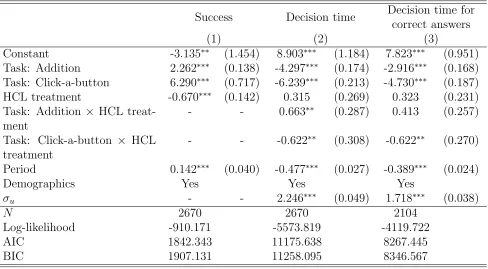
Table 6: Logit regression of success/failure in the decision task and Censored regression of decision time

Success Decision time Decision time for correct answers

(1) (2) (3)

Constant -3.135∗∗ _{(1.454) 8.903}∗∗∗ _{(1.184) 7.823}∗∗∗ _(0.951)

Task: Addition 2.262∗∗∗ _{(0.138) -4.297}∗∗∗ _{(0.174) -2.916}∗∗∗ _(0.168)

Task: Click-a-button 6.290∗∗∗ _{(0.717) -6.239}∗∗∗ _{(0.213) -4.730}∗∗∗ _(0.187)

HCL treatment -0.670∗∗∗ _{(0.142) 0.315 (0.269) 0.323 (0.231)}

Task: Addition × HCL treat-ment

- - 0.663∗∗ _{(0.287) 0.413 (0.257)}

Task: Click-a-button × HCL treatment

- - -0.622∗∗ _{(0.308) -0.622}∗∗ _(0.270)

Period 0.142∗∗∗ _{(0.040) -0.477}∗∗∗ _{(0.027) -0.389}∗∗∗ _(0.024)

Demographics Yes Yes Yes

σu - - 2.246∗∗∗ (0.049) 1.718∗∗∗ (0.038)

N 2670 2670 2104

Log-likelihood -910.171 -5573.819 -4119.722

AIC 1842.343 11175.638 8267.445

BIC 1907.131 11258.095 8346.567

Notes: Standard errors in parentheses. * p<0.1, ** p<0.05 *** p<0.01. Base category is the multiplication task.

13

This is because the HCL treatment is interacted with task dummies and multiplication is the base/excluded task.

14

All in all, the results presented in this section show that the treatment was effective in inducing the desired effect according to our manipulation check. A significant effect shows up even in the task where low reasoning is required (addition task) but not in a task where no reasoning is required (click-a-button task). Furthermore, we found that the effect increases in magnitude in a task involving high reasoning such as the multiplication task.

4.3

Economic rationality

Given that the manipulation checks in section 4.2 show that the cognitive load treatment concurrently affects tasks that involve both low and high reasoning, we now turn to examining the treatment effects for economic rationality. For this, we employ as the dependent variable of interest the various goodness-of-fit measures discussed in Section 3.

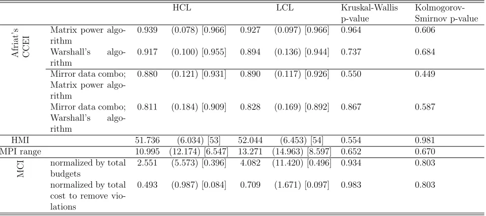
Table 7 shows the mean, standard deviation, and median values for the various measures separately for each treatment. Overall, our calculated goodness-of-fit measures for rationality compare well with other similar experimental studies. For example, average Afriat’s CCEI in

Choi et al.(2014) is 0.881 with a 0.14 standard deviation and a 0.93 median value. The median HMI is 23 (out of 25 choices) in Choi et al. (2014) which compares well with our HMI of 53 and 54 (out of 60 choices) for the HCL and LCL treatments, respectively. The MPI comes in interval form (minimum/maximum) so we employ the range as our dependent variable to use in the table. Table 7 shows that both mean and median values are very close. The last two columns in Table 7 present results from the statistical tests comparing the two treatments. Every single test fails to reject the null indicating a null treatment effect. In addition, Figure 3

graphs the distribution of the various measures by treatment using kernel density estimators. A similar picture emerges since the lines practically overlap for the two treatments.

Figure 3: Kernel density estimators of goodness-of-fit measures for consistency with the Gen-eralized Axiom of Revealed Preference

(a) Afriat’s CCEI (matrix power algorithm) (b) Afriat’s CCEI (Warshall’s algorithm)

(c) HMI (d) MPI range

(e) MCI (normalized by total budgets) (f) MCI (normalized by total cost to remove violations)

Table 7: Descriptive statistics of goodness-of-fit measures by treatment

HCL LCL Kruskal-Wallis

p-value Kolmogorov-Smirnov p-value Af ri at ’s C C E

I Matrix power algo-_rithm 0.939 (0.078) [0.966] 0.927 (0.097) [0.966] 0.964 0.606

Warshall’s algo-rithm

0.917 (0.100) [0.955] 0.894 (0.136) [0.944] 0.737 0.684

Mirror data combo; Matrix power algo-rithm

0.880 (0.121) [0.931] 0.890 (0.117) [0.926] 0.550 0.449

Mirror data combo; Warshall’s algo-rithm

0.811 (0.184) [0.909] 0.828 (0.169) [0.892] 0.867 0.587

HMI 51.736 (6.034) [53] 52.044 (6.453) [54] 0.554 0.981

MPI range 10.995 (12.174) [6.547] 13.271 (14.963) [8.597] 0.652 0.670

M

C

I _{normalized by total}

budgets

2.551 (5.573) [0.396] 4.082 (11.420) [0.496] 0.934 0.803

normalized by total cost to remove vio-lations

0.493 (0.987) [0.084] 0.709 (1.671) [0.097] 0.983 0.803

Table 8: OLS regressions of goodness-of-fit measures and Interval regression (for MPI) with clustered standard errors

Afriat’s CCEI HMI MPI MCI normalized by . . . Matrix

Power algorithm

Warshall’s algorithm

total budget total cost

(1) (2) (3) (4) (5) (6)

Constant 0.733∗∗∗ _0.638∗∗∗ _41.696∗∗∗ _{1.321 16.692 3.361}

(0.135) (0.183) (9.464) (0.933) (14.043) (2.133) HCL treatment 0.015 0.025 -0.156 0.044 -1.245 -0.196

(0.015) (0.020) (1.044) (0.099) (1.549) (0.235) Age 0.005 0.008 0.185 -0.021 -0.531 -0.100

(0.005) (0.007) (0.372) (0.037) (0.552) (0.084) Females -0.016 -0.025 -0.473 0.052 0.462 0.080

(0.014) (0.019) (1.005) (0.093) (1.492) (0.227) Household size 0.003 0.002 0.053 0.044 0.162 0.017

(0.007) (0.009) (0.464) (0.041) (0.689) (0.105) Reference

in-come

-0.000 -0.003 -0.268 0.007 0.272 0.032

(0.005) (0.006) (0.325) (0.031) (0.482) (0.073) Raven’s test

score

0.010∗∗ _0.013∗∗ _0.866∗∗∗ _{-0.048 -0.526 -0.104}

(0.005) (0.006) (0.320) (0.035) (0.475) (0.072) Experience with

Raven’s test

-0.021 -0.032∗ _-1.762∗ _{0.110 2.435 0.363}

(0.014) (0.019) (1.004) (0.098) (1.490) (0.226) Total decision

time

0.000 0.000 0.004 -0.000 -0.001 -0.000

(0.000) (0.000) (0.003) (0.000) (0.005) (0.001)

ln(σ) - - - -0.966∗∗∗ _-

-- - - (0.095) -

-N 178 178 178 178 178 178

R2

0.065 0.076 0.083 0.042 0.049 Adjusted R2

0.020 0.032 0.039 -0.003 0.004

Log-likelihood - - - -217.795 -

-AIC - - - 455.590 -

-BIC - - - 487.408 -

4.4

Was sample size large enough to detect treatment effects?

In this last section of the results we address whether our null effect is genuine. One could rightly ask the question about what is the effect size that our sample size was powerful enough to detect. Or alternatively, whether we could attribute our null result to a false negative.

Our per treatment sample size was decided based on sample size calculations and served as a stopping rule for this experiment when we achieved the necessary per treatment sample. Assuming α = 0.05 (Type I error) and β = 0.20 (Type II error), the per group (treatment) minimum sample size required to compare two means µ0 and µ1, with common variance of σ2

in order to achieve a power of at least 1−β is given by (Kupper and Hafner, 1989):

n= 2(z1−α/2+z1−β)

2

(µ0−µ1

σ )

2 (1)

For α = 0.05 and β = 0.20 the values of z1₋α/2 and z1₋β are 1.96 and 0.84, respectively;

and 2(z1₋α/2+z1_−β) = 15.68, which can be rounded up to 16. The formula then collapses to

n = 16

∆2 (with ∆ =

µ0₋µ1

σ ), which is known as Lehr’s (1992) equation (see also Chapter 2 in

van Belle, 2008). To calculate a minimum sample size, one needs to feed the above formula with values for σ and the minimum meaningful difference µ0 −µ1. To specify the necessary

parameters to feed the above formula, we looked at prior data collected by Choi et al. (2014). Since our induced budget allocation task was based on their study, it seemed natural to use parameter values from theChoi et al. (2014) study. In their paper they calculated both Afriat’s CCEI and the HMI. Panels A and C in Table 1 in Choi et al.’s (2014) online Appendix provided us with the necessary information. For the CCEI, we used a range of σ values from 0.12 to 0.16 (which largely reflects the standard deviations of the CCEI in their study) and a range of possible differencesd from 0.05 to 0.1. For the HMI, we usedσvalues from 2 to 2.4 and a range of possible differences d from 1 to 3.

Table 9: Per treatment sample size calculations for different values ofσ, anddfor Afriat’s CCEI (top panel) and the HMI (bottom panel)

σ = 0.12 σ = 0.14 σ= 0.16

Afriat’s CCEI

d= 0.05 90 123 161

d= 0.06 63 85 112

d= 0.07 46 63 82

d= 0.08 35 48 63

d= 0.09 28 38 50

d= 0.1 23 31 40

σ = 2 σ= 2.2 σ = 2.4

HMI

d= 1 63 76 90

d= 2 16 19 23

d= 3 7 8 10

4.5

Economic rationality, stochastic dominance and risk preferences

Choi et al.(2014) note that consistency with revealed preference theory is a necessary but not sufficient condition for any choices to be considered of high decision-making quality. Although a utility function that rationalizes observed choices might exist, it is not necessary that this function is always normatively appealing. For example, always allocating all points to the same account implies that points will be allocated to the more expensive account in some cases. However, this involves a violation of monotonicity with respect to first-order stochastic dominance.

To account for the extent of GARP violationsand violations of stochastic dominance, Choi et al. (2014) combine the actual data from their experiment and the mirror image of these data obtained by reversing the prices and the associated allocation for each observation. Figure 4

depicts a case where an individual chooses a bundle x1 from the budget line AC with slope

−py/pz (wherepy,pz are the prices of the y and z accounts respectively) and the mirror image

of this choice which is bundle x′1 from the budget line A′C′ with slope−pz/py. The choice ofx1

generates a revealed preference violation involving the mirror image of this decision. However, the choice of x2 does not generate a violation when combined with its mirror image x′2.

statistical tests shown in the same table rejects the null of no difference between the cognitive load treatments. In addition, when we regress Afriat’s CCEI computed over the combined data on the set of regressors shown in Table8, the associated coefficients for the HCL treatment dummy are not statistically significant at conventional significance levels (b =−0.008,p-value = 0.694 for Afriat’s CCEI using the Matrix Power algorithm; b = −0.014,p-value = 0.633 for Afriat’s CCEI using the Warshall’s algorithm).

Castillo et al. (2017) use an alternative measure based on expected payoff calculations and explore, among other things, adherence to payoff dominance in the context of the induced budget line allocation task. Since accounts in the budget allocation task are perfect substitutes (i.e., each account has a 50% probability of being selected as binding), a subject choosing a bundle that is not on the 45◦ _{line (i.e., line z = y in Figure 4) is always better off choosing}

a bundle on the long side of the budget line AC; i.e., on segment BC. On the other hand, choosing a bundle on the short side of the budget line AC; i.e. on segment AB, would violate payoff dominance because the expected payoff is higher for any bundle on the BC segment. To make this more concrete, bundle x1 in Figure 4 violates payoff dominance while bundle x2 does not violate payoff dominance. With our data, we calculate that 33.31% of all choices

were payoff dominated in the LCL treatment and 34.20% were payoff dominated in the HCL treatment. The number of payoff dominated choices is similar to Castillo et al. (2017) where they find that payoff dominance is violated roughly 1/3 of the times. Based on the contingency table of payoff dominant and dominated choices for each treatment, a χ2

text fails to reject the null of no difference between the treatments (χ2

= 0.940, p-value = 0.332). A logit regression (dependent variable is binary: dominant or dominated choice) with clustered standard errors at the individual level, using the same set of regressors reported in Table 8 returns an estimated coefficient for the HCL treatment dummy that is not statistically significant at conventional significance levels (b= 0.056,p-value = 0.492).

Figure 4: Mirror image budget line preference violations

y z

z =y

B

x′1 x′2

A′

C′

x1

x2

A

C

Notes: An individual choosing bundlex1 from the budget line AC with slope−py/pz and the

mirror image bundle x′1 from the budget line A′C′ with slope −pz/py would have violated

GARP. There is no violation of GARP for the bundlex2 and its mirror imagex′2.

With our data, we find that subjects allocate on average 48.64% of the points to the cheaper account under the HCL treatment and 49.84% under the LCL treatment (these numbers imply high levels of risk aversion). A Kruskal-Wallis test fails to reject the null of no difference between allocation of points between the cognitive load treatments (χ2

= 0.199, p-value = 0.656). A regression (dependent variable is percent of points allocated to the cheaper account) with clustered standard errors at the individual level using the same set of regressors reported in Table 8 returns an estimated coefficient for the HCL treatment dummy that is not statistically significant at conventional significance levels (b =−0.012,p-value = 0.308).

Taken together, the results we report in this section are important for a couple of reasons. First, they are relevant because our results show that the null effect we report in the paper is robust even when we account for violations of stochastic dominance. Second, our null effect on risk preferences contrasts that of previous studies: Deck and Jahedi (2015) andGerhardt et al.

5

Conclusions

One important question in economics is whether economic rationality can be influenced by cognitive ability to the extent that inconsistencies resulting from low decision-making quality are due to limited cognitive resources. A number of papers have found that increasing cognitive load can influence performance in reasoning and math tasks as well as risk-aversion and impatience over choices (see Deck and Jahedi,2015). With the exception ofCastillo et al.(2017), no other study has examined the effect of cognitive load on economic rationality.

In our study, we exogenously impaired subjects’ cognitive resources via cognitive load by using a number memorization task. We designed several incentivized manipulation checks to undoubtedly show the success of our manipulation. We then examined the effect of our ma-nipulation on consistency in economic rationality using induced budget allocation tasks and several goodness-of-fit measures for rationality. Our results generally suggest a statistically and economically non-significant effect of cognitive load on economic rationality. We then showed that our study has a large enough sample size, given a power of 80%, to detect even small effects, which suggests that our null effect finding is genuine and not due to false negatives. In-terestingly, a measure of cognitive ability (i.e., the Raven test score) was statistically significant in our regression models suggesting that fluid intelligence could be a more important correlate of economic rationality than temporary cognitive loads in the working memory of subjects. Furthermore, our null result is robust when we account for violations of stochastic dominance that may occur when subjects are asked to choose a bundle on the induced budget line allo-cation task. Importantly, we also find that cognitive load does not generate any breakdown of rationality and does not change risk preferences, in contrast to other (somewhat mixed) results reported in the literature (Castillo et al., 2017; Deck and Jahedi,2015; Gerhardt et al., 2016).

Our finding corroborates well with findings in Deck et al. (2017) where they also find no effect of cognitive load on allocation decisions on money for self and others and suggests that subjects with less cognitive resources could still optimally allocate their limited attention to be-havioral aspects related to economic rationality, akin perhaps to the assumption behind rational inattention models (Sims,2003,2006).

system more, i.e., ‘System 2’. Of course, this was not always effective since, for example, in a high reasoning multiplication task, success rates were particularly low even though subjects took more time answering the multiplication task. Limiting the time subjects could take when making allocations in the budget task, e.g., when under time pressure, is another way one could force engagement of ‘System 1’ and further disengagement of ‘System 2’.

References

Afriat, S. N. (1967). The construction of utility functions from expenditure data. International Economic Review 8(1), 67–77.

Afriat, S. N. (1972). Efficiency estimation of production functions. International Economic Review 13(3), 568–598.

Andreoni, J., M. A. Kuhn, and C. Sprenger (2013). On measuring time preferences. Working paper, University of California at San Diego.

Becker, G. S. (1962). Irrational behavior and economic theory. Journal of Political Econ-omy 70(1), 1–13.

Benjamin, D. J., S. A. Brown, and J. M. Shapiro (2013). Who i