Munich Personal RePEc Archive
Granger causality testing in
mixed-frequency Vars with possibly
(co)integrated processes
Hecq, Alain and Goetz, Thomas
Maastricht University, Deutsche Bundesbank
27 June 2018
Online at
https://mpra.ub.uni-muenchen.de/87746/
Granger causality testing in
mixed-frequency VARs with possibly
(co)integrated processes
Thomas B. G¨otz
∗1and Alain W. Hecq
†21
Deutsche Bundesbank
2Maastricht University
June 27, 2018
Abstract
We analyze Granger causality testing in mixed-frequency VARs with possibly (co)integrated time series. It is well known that conducting inference on a set of parameters is dependent on knowing the correct (co)integration order of the processes involved. Corresponding tests are, however, known to often suffer from size distortions and/or a loss of power. Our approach, which boils down to the mixed-frequency analogue of the one by Toda and Yamamoto (1995) or Dolado and L¨utkepohl (1996), works for variables that are stationary, integrated of an arbi-trary order, or cointegrated. As it only requires an estimation of a mixed-frequency VAR in levels with appropriately adjusted lag length, after which Granger causal-ity tests can be conducted using simple standard Wald test, it is of great practical appeal. We show that the presence of non-stationary and trivially cointegrated high-frequency regressors (G¨otz et al., 2013) leads to standard distributions when testing for causality on a parameter subset, without any need to augment the VAR order. Monte Carlo simulations and two applications involving the oil price and consumer prices as well as GDP and industrial production in Germany illustrate our approach.
JEL Codes: C32
JEL Keywords: Mixed frequencies; Granger causality; Hypothesis testing, Vector autoregressions; Cointegration
∗Thomas B. G¨otz, Deutsche Bundesbank, Economics Department, Macroeconomic
Analy-sis and Projection Division, P.O. Box 100602, 60006 Frankfurt am Main, Germany. Email: [email protected]; the views expressed in this paper are solely ours and should not be inter-preted as reflecting the views of the Deutsche Bundesbank.
†Alain W. Hecq, Maastricht University, School of Business and Economics, Department of Quantitative
1
Introduction
“The world is mixed-frequent” a young researcher said when presenting his paper on forecasting with a mixed-frequency (MF) time series model.1 It not only shows that
MF models constitute a popular and widely studied topic in time series econometrics, it is simply an omnipresent fact applied and theoretical researchers need to deal with, and they do: by now, it has become standard to properly account for the mismatch in publication frequencies among (macroeconomic) time series, instead of aggregating high-frequency (HF) observations using predetermined aggregation schemes (Silvestrini and Veredas, 2008). The set of MF models ranges from single-regression models (e.g., the, by this time, routinely used MIDAS model; see Ghysels et al., 2004 or Ghysels et al., 2007 and, for the unrestricted version, Foroni et al., 2015b) over factor models (see Mariano and Murasawa, 2003, Marcellino and Schumacher, 2010 and Blasques et al., 2016) to vector autoregressive (VAR) models (see, most notably, Ghysels, 2016, Schorfheide and Song, 2015 and Chiu et al., 2011).2
Particularly the latter model class, MF-VAR models, has received a lot of attention recently, predominantly in two related fields of application: forecasting (Schorfheide and Song, 2015 and G¨otz and Hauzenberger, 2017, among others) and Granger causality testing (Ghysels et al., 2016, G¨otz et al., 2016 and Ghysels et al., 2017). Both topics are of immense interest to practitioners at, e.g., central banks, who routinely forecast key variables like the gross domestic product (GDP) using a variety of, usually higher-frequent, indicators, or investigate causal patterns between the time series they monitor. We will focus on Granger causality (GC) testing, generally introduced in Granger (1969), whereby both concepts are obviously related due to the way GC is usually defined. The three papers mentioned above cover different aspects of GC testing within a MF-VAR: Ghysels et al.
1Unfortunately, the name of said researcher as well as the conference he presented at slipped the
authors’ memories; as if choosing the adjective “young” was not enough for proving that one grew older.
2There exists a multitude of sub-variants of each model class, e.g., hybrid versions of MIDAS LASSO
(2016) discuss the general theory of associated hypothesis tests in detail, which – while asymptotically valid – suffer from size distortions and a loss of power in case the number of HF observations is large relative the low-frequency (LF) period. G¨otz et al. (2016) and Ghysels et al. (2017) then introduce various ways to overcome these implications of the curse of dimensionality. Yet, all three papers have one assumption in common, i.e., they
remain in a stationary time series environment after properly transforming the series; in this paper we allow the variables to be integrated or cointegrated.
If we knew the order of integration of the variables under consideration as well as whether the series are cointegrated, we could transform an initial MF-VAR in levels to a model in differences or to an error correction model (ECM) and test for GC using the methods of Ghysels et al. (2016) or G¨otz et al. (2016) and Ghysels et al. (2017), depending on the frequency mismatch. In practice, though, we usually do not know the precise (co)integration order, and appropriate tests are required beforehand; tests that – in the case of unit roots – tend to have rather low power or that – in the case of cointegration – may suffer from severe size distortions (Ghysels and Miller, 2015). Instead of testing for GC in a system, that is a-priori transformed based on the outcomes of more or less error-prone pre-tests, we aim at a methodology that allows estimation of the MF-VAR in levels and leads to valid and standard inference procedures.
show that for the stacked, observation-driven MF-VAR system of Ghysels (2016),3 the
necessary adjustment is small at worst and in some cases even entirely superfluous. This causes the corresponding inefficiencies to be lower than in the common-frequency case or to be absent altogether.
To be more precise, and to highlight the most important consequence of our approach, consider testing for GC from a high- to a low-frequency variable, i.e., the arguably more in-teresting case in terms of nowcasting a LF series (e.g., quarterly GDP) using HF indicators with eventual leading properties (e.g., monthly surveys). Using our simple methodology one can apply a standard Wald test on a MF-VAR estimated in levels without any need to adjust the lag length, irrespective of the (co)integration order of the series involved. Key for this finding is the presence of “trivial” cointegrating relationships among the stacked HF series (G¨otz et al., 2013) and a suitable application of Theorem 1 of Toda and Phillips (1993). With respect to testing the reverse direction, only a small adjustment of the system suffices to rely on an asymptoticχ2-distribution.
The rest of the paper is organized as follows. In Section 2 we describe the model, introduce GC testing within the MF-VAR and outline the different augmentations en-suring valid inference in levels, irrespective of the order of (co)integration. We present the theoretical background for our approach and confirm our findings using Monte Carlo simulations in Section 3. An empirical analysis in Section 4 illustrates our approach for German data involving the consumer price index and the oil price as well as GDP and industrial production. Section 5 concludes.
3We leave an analysis of the same research question for parameter-driven MF-VAR models `a la
2
GC Testing in MF-VARs
2.1
The Model
Let us assume a two-variable MF system, where yt represents the LF variable running
from t = 1, . . . , T. The HF variable x appears m times as often, implying m = 3 for a month/quarter- or m = 4 for a quarter/year-example. We writex(tm−i/m) for a specific HF
observation, whereby i = m−1 (i = 0) represents the beginning (end) of a LF period
t. The LF and HF lag and difference operators are denoted Li and ∆i as well as Lj/m
and ∆j/m, respectively. Hence, ∆iyt=yt−Liyt =yt−yt−i and ∆j/mxt=xt−Lj/mxt =
xt−xt−j/m. Also, L1/mxt−(m−1)/m =xt−1. For this rather standard notation in the MF
literature, see also Clements and Galv˜ao (2008) or Miller (2014). Furthermore, we denote an integrated process of integer order d by I(d) and a cointegrated process of order d, b
byCI(d, b). Finally, vecrepresents the operator stacking the columns of a matrix, ⊗ the Kronecker product, Ik the identity matrix of dimension k and 0i×j an (i×j)-matrix of
zeros.
Remark 1 In principle, we could allow for higher dimensional multivariate systems by,
e.g., consideringnl LF andnh HF series, where the HF series may have different sampling
frequencies mj, j = 1, . . . , nh. Firstly, though, analyzing GC in a system with more than
two variables opens the door for multi-horizon causality and thus to causal chains (see,
e.g., L¨utkepohl, 1993). Secondly, such an extension would complicate the notation and
illustration of results.
The observation-driven MF-VAR of Ghysels (2016) is constructed by first stacking the HF observations corresponding to one t-period together with the observation for y
yielding Zt= (yt, X(m)
′
t )
′
, whereXt(m)= (xt(m), x(t−m1)/m, . . . , x
(m)
t−(m−1)/m) ′
. Then, a dynamic structural equations model for Z can be written as
AcZt=A
∗
1Zt−1 +. . .+A ∗
pZt−p+u ∗
where coefficients in Ac govern the evolution within the HF process x as well as
so-callednowcasting causality (G¨otz and Hecq, 2014). u∗
t is an independently and identically
distributed (i.i.d.) error term with E(ut) = 0(m+1)×1, E(u ∗
tu
∗′
t) = Σu∗, the latter being a
diagonal matrix of dimension m+ 1 with (1,1)-element σ2
y and σ2x (the variances of the
processes y and x) on the remainder of the diagonal. After pre-multiplying (1) by A−1
c
we obtain the reduced-form MF-VAR(p):
Zt=A1Zt−1+. . .+ApZt−p +ut =AZ−p+ut (2)
withAj =A−c1A
∗
j, j = 1, . . . , p,,ut=A−c1u
∗
t,A= (A1, . . . , Ap) andZ−p = (Z ′
t−1, . . . , Z ′
t−p) ′
. Note that we exclude an intercept, mostly for ease of notation.4 Let us make the following
assumptions:
Assumption 1 Ztis generated by the MF-VAR(p) in (2), whereby (i)ZtisI(d)and may
or may not be CI(d, b); ut is an i.i.d. sequence of (m+ 1)-dimensional random vectors
with E(ut) = 0(m+1)×1, E(utu ′
t) = Σu, where Σu > 0 such that E|ujt|2+δ < ∞ for some
δ >0.
Remark 2 As in Toda and Yamamoto (1995) and Dolado and L¨utkepohl (1996), we
initially assume the lag order p to be a-priori known or estimated via some standard selection criterion. Indeed, one may expect biases resulting from such pre-tests to affect
all approaches more or less equally.
Remark 3 As far as the difference in frequencies between y and x, captured by the pa-rameter m, is concerned, we primarily focus on rather small values, i.e., m≤4. Firstly, the corresponding cases are usually of more interest in typical macroeconomic
applica-tions (see, e.g., Section 4). Secondly, the size of the MF-VAR in (2) grows rapidly with
m. Consequently, inefficiencies resulting from the inherent curse of dimensionality will most likely dominate any effects from testing for GC using one or the other approach.
4One may think of the processes to be demeaned a-priori. As in Dolado and L¨utkepohl (1996), the
Thirdly, small values of m allow us to rely on standard asymptotic theory for Wald test (Ghysels et al., 2016), even in the benchmark case.5
Remark 4 Assumption 1 implies that the data are truly generated at mixed frequencies.
Alternatively, one could base the analysis on a common HF data generating process (DGP)
and obtain model (2) by temporally aggregating the LF series (see, inter alia, Ghysels and
Miller, 2015, Zadrozny, 2016 or Koelbl and Deistler, 2018). Our goal, however, is not to
study which causality patterns can be preserved when moving from a latent HF system to a
MF one,6 but to find an asymptotically valid approach to conduct inference in a model that
is directly estimable by practitioners. Additionally, we base our analysis on a model with
observable data only, not involving latent processes of any kind. Such parameter-driven
MF-VAR models (see, e.g., Schorfheide and Song, 2015) certainly have their merits, but
do not lend themselves easily to a (co)integration-order-robust way of GC testing. The
model in (2), however, does, which is why we consider that model whenever we refer to a
MF-VAR.
2.2
Standard Approach
GC testing within a MF-VAR boils down to testing a set of zero restrictions on the coefficient matrices A= (A1, . . . , Ap). In particular, testing for Granger non-causality in
both directions implies testing the following null hypotheses in system (2):
HHF9LF
0 :A (1,2)
i =A
(1,3)
i =. . .=A
(1,m+1)
i = 0 ∀i= 1, . . . , p, (3)
HLF9HF
0 :A (2,1)
i =A
(3,1)
i =. . .=A
(m+1,1)
i = 0 ∀i= 1, . . . , p, (4) 5One could – as mentioned above – rely on the approaches of G¨otz et al. (2016) or Ghysels et al.
(2017) in casemis comparably large. However, the performance of these tests in a situation, where the (co)integration order of the variables is unknown, is unclear and should be inspected first.
6In fact, as shown by Ghysels et al. (2016), depending on the aggregation scheme used, Granger
where A(ir,c) denotes the (r, c)-element of matrix Ai.7 Of course, if we knew the process
Z to be I(0), we could just estimate model (2) in levels and apply a standard Wald test: for ap = vec(A1, . . . , Ap) and a suitably constructed matrix R, we can rewrite both null
hypotheses as
H0 :Rap =0mp×1
and compute the Wald statistic as
W = (Rˆap)
′
(RΩˆR′
)−1
(Rˆap)
with ˆΩ = (A′
A)−1
⊗Σˆu and ˆΣu = (ˆu′uˆ)/(T −p) being a consistent estimator of Σu. For
a stationary MF-VAR, Ghysels et al. (2016) show the Wald statistic to be asymptotically
χ2(mp)-distributed. We refer to testing for GC in this way as “standard test”.
In case we knew the process Zt to be I(d), we could achieve stationarity of the
MF-VAR by differencing d times. Here, however, an additional ambiguity is added to the situation due to the presence of mixed frequencies: while LF differences are surely being applied toy, one could either use ∆ or ∆1/mfor x. Indeed, both transformations applied
d times yield a stationary process, yet have consequences on the dynamics of the system and thereby on conducting inference. Somewhat similarly, in the additional presence of cointegration between y and x we can follow the lines of either G¨otz et al. (2013) or Ghysels and Miller (2015), who derived alternative specifications of a MF-VECM.8 Again,
which specification is chosen in the end has implications for the construction of GC tests and may affect their performance, especially in finite samples. At the very least, it affects the way in which trivial cointegrating relationships among the HF series themselves enter the model (G¨otz et al., 2013).
Obviously, the (co)integration orders of the series are not known a-priori and a battery
7The alternative hypotheses, of course, imply that at least one of the respective coefficients is non-zero. 8For the single-regression counterpart Miller (2014) and G¨otz et al. (2014) developed MF-ECMs,
of pre-tests are usually performed. With respect to tests for the order of integration (usually the ones based on Dickey and Fuller, 1979, Phillips, 1987 or Phillips and Perron, 1988),9 however, power tends to be rather low against a (trend) stationary series. As
for tests on cointegration, Ghysels and Miller (2015) show that depending on the (often unknown) aggregation scheme underlying the series, one may have to expect severe size distortions.10 Given the pitfalls of such pre-tests, an approach for GC testing in levels
irrespective of the (co)integration orders of the variables would be highly valuable.
Remark 5 Like Dolado and L¨utkepohl (1996), we focus ond= 1in this paper to simplify notation and discussion. On the one hand it is indeed the most important case in practice,
on the other hand the approach and theory extend quite straightforwardly to d > 1 (see Toda and Yamamoto, 1995 for the common-frequency case). We will mention any changes
due to larger d in footnotes.
2.3
TY/DL Approach
In the common-frequency framework, Toda and Yamamoto (1995) as well as Dolado and L¨utkepohl (1996) show the following simple strategy to achieve the desired outcome: instead of transforming the VAR, estimate it in levels, but augment the regressor set by an additional lag, i.e., Zt−(p+1). Subsequently, test for Granger non-causality on the original
coefficients (corresponding toZt−1, . . . , Zt−p) in the modified model. The reason why this
approach leads to valid inference, also for I(1) process that are not cointegrated, goes back to an early contribution by Sims et al. (1990). They showed that parameters that can be re-written as coefficients on zero-meanI(0) regressors, have a standard asymptotic distribution. Here, it is important to notice that one does not need to re-write the model
9Note that as such tests are done for each variable individually, the MF nature of the variables plays
a minor role here.
10To be precise, if the variables are aggregated with identical schemes (e.g., both end-of-period sampled
accordingly, it is enough if it is theoretically possible to do so.
Providing more practical appeal to this result, let us consider the situation of common-frequency VAR, where ZCF
t = (yt, xt)′ is I(1) and CI(1, b) for some b. A well-known
way to re-write this model in accordance with the finding of Sims et al. (1990) is the ECM format: due to cointegration, all coefficients (which are transformations of the parameters in the original VAR in levels) are assigned to stationary regressors. In the absence of cointegration, however, one of the regressors (depending on how we transform the original model, i.e., which lag i ∈ 1, . . . , p we capture the long-run term with) will remain I(1). Now, imagine we add Zt−(p+1) to the VAR in levels and re-write the model
as follows:
ZtCF = Ppi=1AiZtCF−i +Ap+1Z
CF
t−(p+1)+εt
⇔∆p+1ZtCF =
Pp
i=1Ai∆(p+1)−iZtCF−i −ΠZ
CF
t−(p+1)+εt,
where Π =I−Ppi=1Aiand ∆jZtCF =ZtCF−ZtCF−j. Hence, no matter whether the series are
cointegrated, the standard Wald test applies to the coefficients corresponding to the first
p (stationary) regressors.11 Said differently – using the terminology in Sims et al. (1990)
or Toda and Phillips (1994) – in case of anI(1) system, one needs “enough cointegration” or additional lags to account for the nondegenerate stochastic trends.
The MF analogue of this approach is thus to replaceZCF
t byZtand estimating the
MF-VAR in levels, thereby obtaining ˆap+1 =vec(A1, . . . , Ap, Ap+1)≡ vec(A∗). The modified
Wald test is then still applied on the mp elements corresponding to the GC-relevant elements in A; in terms of null hypothesis and Wald test:
H∗
0 : R
∗
ap+1 =0mp×1,
W∗
= (R∗
ˆ
ap+1)′(R∗Ωˆ∗R∗′)−1(R∗ˆap+1),
11We refer to Dolado and L¨utkepohl, 1996, p. 372 for this illustrating example and Theorem 1 of the
where ˆΩ∗
= (A∗′
A∗
)−1
⊗Σˆ∗
u and ˆΣ∗u being a consistent estimator of the covariance matrix
in the modified MF-VAR. We refer toW∗
based on Toda and Yamamoto (1995) or Dolado and L¨utkepohl (1996) as “TY/DL-test”.
Of course, the robustness of the TY/DL-test to the (co)integration order of the system does not come freely. Intentionally over-fitting the model in this way quickly leads to inefficiencies in case the adjustment is not necessary. This cost is obviously higher in a MF-VAR as an extra lag adds (nl + mnh)2 (in the two-variable system (m + 1)2)
coefficients to be estimated. But there are ways to decrease these costs or to get rid of them altogether...
2.4
Mixed-Frequency Approach
Under the null hypothesis, it is clear that one cannot do better than designing an asymp-totically valid inference method. While the TY/DL-test does so irrespectively of the (co)integration order of the series involved, it may – in small samples – suffer from size distortions and inefficiencies by intentionally over-fitting the model. We aim for an ap-proach that may keep such issues at bay, while still providing an asymptotically valid test. We propose two approaches: the “MF-dep-test”, indicating that this procedure depends on the GC testing direction, and an alternative “MF-indep-test”.
2.4.1 MF-dep-test
Testing HHF9LF
0 : We start by considering the test direction from the high- to the
low-frequency series, i.e., the arguably more interesting case in practice given that one is often interested in evaluating the effects of a HF indicator (e.g., a survey variable) on a LF aggregate (e.g., GDP). We propose the following procedure:
• Estimate the MF-VAR in (2) in levels and obtain ˆap as in Section 2.2, i.e., without
augmenting the system with an additional lag.
two Wald statistics corresponding to (i) the (1,2)-element of each autoregressive matrix being equal to zero and (ii) the (1,3) up to (1, m+ 1)-elements of each A -matrix being jointly equal to zero.12 For accordingly constructed selection matrices
RHF1 and RHF2, this boils down to
H0HF1 : RHF1a
p =0p×1,
HHF2
0 : RHF2ap =0p(m−1)×1,
WHF j = (RHF jˆa
p)′(RHF jΩˆHF jRHF j′)−1(RHF jaˆp)
for j = 1,2 and properly constructed matrices ˆΩHF j.
• Compare the correspondingp-values of theχ2(p)- andχ2(p(m−1))-distributed test
statistics to α/2, where α represents the significance level, i.e., apply a Bonferroni correction to account for the fact that we want test both null hypotheses jointly (Dunn, 1961).
• RejectH0HF9LF if you rejectH0HF1,H0HF2or both; otherwise do not rejectH0HF9LF.
In this case, we can hold on to the original model in (2), i.e., no intentional over-fitting is necessary! This means we can stick to the usual and simple MF-VAR(p) model in levels, a remarkably convenient outcome, especially for applied work. Hopefully avoiding eventual inefficiencies comes at a rather cheap price: all we have to do is compute two Wald statistics instead of one.
The intuition for this finding rests on the fact that the stacked VAR structure provides us with “enough [or] sufficient cointegration”, in the sense of Toda and Phillips (1994). To be more precise, the HF variables – provided they areI(1) – are trivially cointegrated with each other, i.e., m −1 cointegrating relationships are a-priori known (G¨otz et al., 2013). Hence, the absence of additional cointegration just forces us to test at mostm−1
12Ford >1, we propose to apply tests on (i) the elements (1,2) up to (1,1 +d) and (ii) the elements
(1, d+ 2) up to (1, m+ 1) of each autoregressive matrix. In cased≥mone does not get around adding
Xt(m)
coefficients at a time.13 Loosely speaking, once could say that we apply the argument of
Toda and Yamamoto (1995) and Dolado and L¨utkepohl (1996) “backwards”: instead of looking at m+ 1 coefficients, of which m are tested on, we look at m and test on m−1 (two times).
Importantly, note in the presence of additional cointegration betweenxandy, the extra cointegrating relationship compensates for the one missing linear combination among the trivial ones; the standard approach, i.e., testing zero restrictions on all m coefficients per autoregressive matrix jointly, would thus have sufficed (L¨utkepohl and Reimers, 1992).
Testing HLF9HF
0 : Let us now consider the reverse test direction, i.e., the one from
the low- to the high-frequency series. Albeit being less common, this situation is still of interest. Apart from being complete on the issue, there are (macro)economic examples such as quarterly capacity utilization rates (e.g., in Germany), which may affect indicators like monthly industrial production. Here is what we propose for this test direction:
• Augment the MF-VAR in (2) by adding the regressor yt−(p+1) to each equation:14
Zt= p
X
i=1
AiZt−i+A
(·,1)
p+1yt−(p+1)+υt
with A(p·+1,1) being an (m+ 1)-vector (the notation resembling the similarity to the first column of matrixAp+1used for the TY/DL-test). Estimate the model in levels,
thereby obtaining ˆap+ 1
m+1 =vec( ˆA1, . . . ,
ˆ
Ap,Aˆ(
·,1)
p+1) = vec(ALF).
• Consider the usual mp GC-relevant coefficients, i.e., the ones appearing in (4). For
an accordingly constructed selection matrix RLF, the null hypothesis and Wald 13Alternatively to splitting the m coefficients as proposed here, one may testm−1 coefficients two
times, once element (1,2) up to (1, m) of eachA-matrix and once elements (1,3) up to (1, m+1). However, the presence of overlapping coefficients makes the subsequent Bonferroni correction overly conservative. Likewise, testing each of themsets of coefficients individually is asymptotically valid, yet complicates a joint consideration of themrespective null hypotheses.
14Generally, i.e., also ford >1, one has to add regressors y
statistic read
H0LF : RLFap+ 1
m+1 =0mp×1,
WLF = (RLFaˆ p+ 1
m+1) ′
(RLFΩˆLFRLF′
)−1
(RLFˆa p+ 1
m+1)
with ˆΩLF = (A(LF)′
A(LF))−1
⊗ΣˆLF
υ , the latter being a consistent estimator of the
covariance matrix in the augmented model.
• Inspect thep-value of theχ2(mp)-distributed test statistic to decide uponH0LF9HF.
Here, the situation is a bit different, because the LF variable y is not part of any trivial cointegrating relationship. Hence, we will not get around performing some sort of adjustment along the lines of the TY/DL-test. Yet, in contrast to how the straightforward extension described in the previous subsection works, we want to limit the amount of over-fitting as much as possible. As we only require yt−(p+1) for being able to re-write
the model in an ECM-fashion (see the example in Section 2.3), we propose to merely add this regressor to each equation of the system. This implies an addition of merely m+ 1 coefficients to be estimated, in contrast to the (m+ 1)2 for the TY/DL-test.
2.4.2 MF-indep-test
In contrast to the approach of Toda and Yamamoto (1995) or Dolado and L¨utkepohl (1996), the MF-dep-test depends on the direction of GC we are interested in. If one aims for GC testing in both directions using the same estimated model, one does not get around an adjustment similar to the TY/DL-test. To be precise, one would need to add at least yt−(p+1) and one HF observation from periodt−(p+ 1), e.g.,x
(m)
t−(p+1). Of course,
2.5
Overview
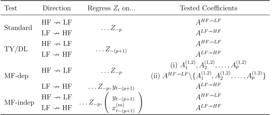
Now that we have introduced each of the potential ways to test for GC in both directions, Table 1 provides a small overview. To this end, revisit the most general reduced-form MF-VAR(p) in (2), i.e., Zt =AZ−p +ut with A = (A1, . . . , Ap) and Z−p = (Z
′
t−1, . . . , Z ′
t−p) ′
, for the vector Zt = (yt, Xt(m))
′
with Xt(m) = (x
(m)
t , x
(m)
t−1/m, . . . , x
(m)
t−(m−1)/m) ′
. Let the set of coefficients corresponding to testing for GC from the HF to the LF series in the standard approach, i.e., the ones in, be denoted as
AHF9LF =A(1,2)
1 , . . . , A(1p,m+1), . . . , . . . , Ap(1,2), . . . , A(1p,m+1),
and likewise for the reverse direction, i.e., the ones in (4),
ALF9HF =A(2,1)
1 , . . . , A (m+1,1)
1 , . . . , . . . , A(2p,1), . . . , A(pm+1,1).
Finally, let “C\D” denote “C without D”.
3
Theoretical Background and Simulations
3.1
Partially cointegrated systems
The validity of the proposed approach in this paper – at least as far as testing the direction from the HF to the LF series is concerned – rests on the theoretical framework in Toda and Phillips (1994), which we revisit here. While our approach for testing the reverse direction may also be validated using similar grounds, the methodology underlying both the MF-dep- and the MF-indep-test is, in fact, broadly identical to the TY/DL-procedure. Hence, we refer to the respective papers in this case.
Recall that we consider a two-variable MF system, where we want to test whether the m series corresponding to the HF variable Granger cause y. Now, let Πθ be the
Given a set of fairly mild assumptions, some of which are already encompassed by the ones we stated at the beginning of Section 2 and the others easily transferable (see Toda and Phillips, 1994, p. 261), the following holds:
Theorem 1 Suppose we are under the following null hypothesis:
H0 :A(1i ,g1) =. . .=A
(1,g2)
i = 0 ∀i
for 2≤g1 ≤g2. Then, if rank(Πθ,g1:g2) =g(≤ng =g2−g1 + 1), we obtain the following
for the corresponding test statistic:
WHF →dχ2(ng(p−1) +g) +✶(g<ng)T N P,
where T N P denotes a term (nonstandard distribution) that depends on nuisance param-eters, that in turn depend on the long-run covariance matrix. Note that T N P cancels for
g =ng, though (labeled using the indicator function).
This Theorem has a series of implications, directly related to our situation. Corrolary 1 shows that the standard approach works even if the series are I(1), provided they are cointegrated. In case cointegration betweenx and yis absent, though, the test converges to a mixture of a chi-square and and a nonstandard distribution, the latter depending on nuisance parameters (Corrolary 2).
Corrolary 1 Suppose there is cointegration between the I(1)-series x and y and we test the entire set of coefficients corresponding to the HF series, i.e., g1 = 2 and g2 =m+ 1,
implying ng = m. Then, as rank(Πθ,2:m+1) = m (see G¨otz et al., 2013) we have that
WHF →dχ2(mp).
Corrolary 2 Suppose there is no cointegration between the I(1)-series x and y and we test the entire set of coefficients corresponding to the HF series, i.e.,g1 = 2andg2 =m+1,
implying ng =m. Then, as rank(Πθ,2:m+1) =m−1 (see G¨otz et al., 2013) we have that
Now, the MF-dep-test rests on computing two Wald statistics, that are subsequently combined using the Bonferroni approach. For each of the individual tests, we have the following for the cointegration- and the no-cointegration-case (Corrolary 3):
Corrolary 3 Suppose the series x and y are I(1) and we test two sets of coefficients corresponding to the HF series: (i) for g1 = 2 and g2 = 2, implying ng = 1 and (ii) for
g1 = 3 and g2 =m+ 1, implyingng =m−1. For (i)rank(Πθ,2:2) = 1 s.t. WHF →d χ2(p)
and for (ii) rank(Πθ,3:m+1) = m−1 s.t. WHF →dχ2((m−1)p).
3.2
Monte Carlo study
3.2.1 Setup
In order to investigate size and power properties of the various test versions in finite sam-ples, we conduct a series of simulation experiments. In particular, we assess the sensitivity of the results with respect to the sample size (T = 50,150,250) and the frequency discrep-ancy (m = 2,3,4). All simulations are based on a 10,000 replications of the respective DGP and plot the rejection frequencies of the test statistics in Table 1.
We start by describing our MF-DGP, i.e., the data are truly generated at mixed frequencies (see Remark 3), flexibly incorporating the different possible features of the data. Due to the potential presence of cointegration, through which GC in one direction is present by construction, we need to differentiate the DGP for both test directions. Hence, let yt and x(tm) be generated by one of the following systems, depending on whether we
inspect...
...GC fromx to y, i.e.,
yt = ρyt−1+
m−1
X
j=0
λj∆xt(−m1)−j/m+ǫy,t, (5)
x(tm−j/m) = θyt+v
(m)
x,t−j/m, where v
(m)
x,t−j/m = (α+ 1)v
(m)
x,t−(j+1)/m+ǫ
(m)
..., or GC from y tox, i.e.,
yt = θx(tm)+vy,t, where vy,t = (α+ 1)vy,t−1+ǫy,t, (7)
x(tm−j/m) = ρx
(m)
t−(j+1)/m+δj∆yt−1+ǫ
(m)
x,t−j/m, (8)
where ǫy,t, ǫ(x,tm−)j/m ∼N(0,1),
15 j = 0, . . . , m−1 and −2≤α ≤0.
Note that (5) contains a U-MIDAS-type (Foroni et al., 2015b) impact of the HF series ony, and that (8) features a similar effect of past LF-differences onx.16 This setup allows
us to look at the consequences of I(1)-ness as well as cointegration simultaneously or in isolation. In case −1 < ρ < 1 (i.e., x or y is I(0) depending on the DGP), the value of
α determines whether the other series is I(0) as well (−2 < α <0) or whether it is I(1) (|α+ 1| = 1). In case |ρ| = 1 (i.e., x or y is I(1) depending on the DGP), α controls the presence or absence of cointegration, respectively. In the cointegrated case, θ then governs the cointegrating relationship.
After some manipulations, both DGPs can be re-written into a reduced-form MF-VAR(2) in levels, i.e.,
Zt=A1Zt−1+A2Zt−2+ut,
where ut = A∗u∗t with u
∗
t = (ǫy,t, ǫ(x,tm), ǫ
(m)
x,t−1/m, . . . , ǫ
(m)
x,t−(m−1)/m) ′
∼N(0m+1×1, Im+1) such
that Σu =A∗′A∗; precise formulae forA1, A2andA∗under both DGPs are being delegated
to Appendix B.
Remark 6 To show that these DGPs nest the case of a cointegrated system with trivial
cointegrating relationships, consider the example of m = 3 and ρ = 1 such that both y
and x are I(1). Using the formulae for A1, A2 and A∗ in the Appendix, the reduced-form
MF-VARs can be re-written into the following VECMs (G¨otz et al., 2013 or Ghysels and
Miller, 2015).
15Hence,σ2
y=σ2x= 1.
16Note that one could leave the impact of the lagged series constant over one t-period, significantly
For GC from x to y, i.e., the DGP in (5) and (6):
∆yt
∆x(3)t
∆x(3)t−1/3
∆x(3)t−2/3
=
0 0 0 0
−θα(α2+ 3α+ 3) α(α2+ 3α+ 3) 0 0
−θα(α+ 2) α(α+ 2) + 1 −1 0
−θα α+ 1 0 −1
| {z }
Π
yt−1
x(3)t−1
x(3)t−4/3
x(3)t−5/3
+
0 λ0 λ1 λ2
0 θλ0 θλ1 θλ2
0 θλ0 θλ1 θλ2
0 θλ0 θλ1 θλ2
∆yt−2
∆x(3)t−2
∆x(3)t−7/3
∆x(3)t−8/3
+ut.
For GC from y to x, i.e., the DGP in (7) and (8):
∆yt
∆x(3)t
∆x(3)t−1/3
∆x(3)t−2/3
=
α −θα 0 0
0 0 0 0
0 1 −1 0 0 1 0 −1
| {z }
Π
yt−1
x(3)t−1
x(3)t−4/3
x(3)t−5/3
+
θ(δ0+ρδ1+ρ1δ2) 0 0 0
δ0 +ρδ1+ρ1δ2 0 0 0
δ0+ρδ1 0 0 0
δ0 0 0 0
∆yt−2
∆x(3)t−2
∆x(3)t−7/3
∆x(3)t−8/3
+ut.
Indeed then, for α = 0 the matrix Π (in both DGPs) merely contains the trivial coin-tegrating relationships among the HF variable itself. For −2 < α < 0, though, there is an additional cointegrating relationship between y and x of the form (−θ,1) or (1,−θ), respectively. To see this, note that one can write Π = ΠαΠθ, where Πα and Πθ are both
relationships.
Now, the null hypotheses for both test directions (under their respective DGP) are easily seen to be:
HHF9LF
0 :λj = 0 ∀j = 0, . . . , m−1,
HLF9HF
0 :δj = 0 ∀j = 0, . . . , m−1.
We will consider three cases: (a)yandxareI(0) by settingρ= 0.8 andα=−0.5, (b)
yandxare I(1) and cointegrated by settingρ= 1 andα=−0.5, (c)yandxareI(1) but not cointegrated by setting ρ = 1 and α = 0. Throughout the simulations, θ = 0.5. We set the GC-determining coefficients to λ=T−0.5
λ∗
for λ∗
={0,1,2}; likewise for δ. Note that values of zero imply no GC (size), whereas non-zero values imply GC (power).17 The
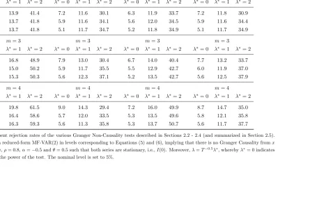
results are summarized in (a) Tables 2 and 3, (b) Tables 4 and 5 and (c) Tables 6 and 7.
3.2.2 Results
The stationary scenario is obviously favourable for the standard test, which is asymptot-ically χ2(mp)-distributed. While incurring some size distortions for small T, it leads to
the correct size for larger sample sizes. Furthermore, this test is the most powerful one for each (T, m, λ∗
/δ∗
)-combination as it is does not feature any alteration to the estimated model. The TY/DL- and the MF-indep-test perform almost identically, the latter having slightly higher rejection rates under the alternative, becausem2−1 fewer parameters need
to be estimated. Compared to the standard test, though, power is clearly inferior. Inter-estingly, the MF-dep-test seems to cope somewhat better with size distortions arising from small T, particularly when testing the empirically more interesting GC-direction from x
toy. Granted, it still falls short of the standard test’s power, yet it beats the TY/DL- and MF-indep-tests, clearly so again for testing HF 9 LF. Overall, the MF-dep-test presents a more than compelling approach for I(0)-MF-series.
17This specification of the GC-determining coefficients is derived from the Monte Carlo study in Dolado
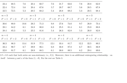
Let us turn to the more interesting cases, in whichxandyare non-stationary, and start with the cointegrated scenario (b). From Corollary 1 it follows that the standard test is in fact still favoured in this situation. Together with the trivial cointegrating relationships among the HF series, the presence of additional cointegration between x and y implies “enough cointegration” (Toda and Phillips, 1994) to yield a χ2(mp)- distribution of the
standard Wald test. As a consequence, the outcomes in Tables 4 and 5 are qualitatively identical to the ones for the stationary case (a) in Tables 2 and 3.
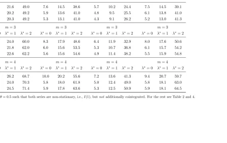
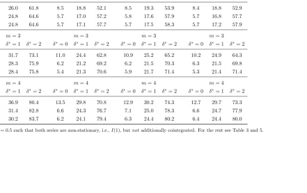
Finally, inspecting the non-stationary and non-cointegrated (w.r.t. xandy) case (c) in Tables 6 and 7 reveals that the standard test does not have aχ2(mp) underH
0 (Corrolary
2). Indeed, even for large T, actual size clearly exceeds the nominal level of 5%. The TY/DL- and MF-indep-tests, on the other hand, constitute asymptotically valid tests, although they are – as before – somewhat oversized for a small sample size. In terms of power, though, they perform rather well, more so given that size-adjusted power of the standard test would surely turn out to be smaller than the size-unadjusted figures presented here.
As far as the MF-dep-test is concerned, let us discuss the outcomes for the two GC test directions separately. For testing GC from y to x the approach is almost identical to the MF-indep-test (and the TY/DL-test for that matter); only that fewer parameters need to be estimated (revisit Section 2.4). In terms of size, the outcomes are thus by and large comparable, whereas power is either as high as or even slightly higher when using the MF-dep-test. For testing GC from x to y, asymptotic validity of the MF-dep-test is also confirmed (see Corrolary 3 and – for the Bonferroni correction – Dunn, 1961), but more noteworthily the test appears far less oversized than its competitors: even for
T = 150 and m = 4 empirical size coincides with the nominal one. The cost of this presumably controlling effect the Bonferroni correction has is a loss of power, which is most pronounced for cases closer to the common-frequency setup, i.e., the smaller m
To sum up, the MF approaches present competitive and easy-to-implement alternatives to the existing TY/DL-approach. Here, the MF-indep-test yields marginally better results throughout the entire analysis, which is not too surprising given the only slight adjustment in test design. The MF-dep-test is mostly the preferred choice, although in the absence of cointegration betweenx andy the merits of a correctly sized test – also for small samples – stand against somewhat lower power. From an empirical and conservative standpoint, however, the MF-dep-test is the dominant strategy.
Remark 7 We also experimented with an alternative, equally accepted way to perceive the
DGP underlying the observable MF data (Ghysels and Miller, 2015, Ghysels et al., 2016 or
Miller, 2014): that the data are all generated at the common HF, yet the ones observable
at the LF contain latent observations. To be more precise, we considered a DGP that is
directly derived from the setup in Dolado and L¨utkepohl (1996) for the common-frequency
case; see Appendix C for explicit formulae. In line with most macroeconomic applications,
we temporally aggregated the mT HF-observations of y using the simple average of the m
values corresponding to each t-period.
While the outcomes were broadly in line with the ones for the MF-DGP as far as GC
fromy toxare concerned (with somewhat lower power, though), the results for testing GC from x to y revealed the shortcomings of such a DGP: as shown by Ghysels et al. (2016), depending on the aggregation scheme, Granger non-causality will not be preserved when
moving from a HF- to a MF-VAR. In particular, “a crucial condition for non-causality
preservation is that the information for the [variable that is caused by the other under
HA, i.e., y] is not lost by temporal aggregation” (p. 216). This condition is only satisfied
in some specific, simple cases and surely not in the scenarios of most interest for us here
(averaging y, I(1)-ness, potential cointegration).18
18The results of the Monte Carlo experiments based on a HF-DGP are not displayed here to save on
4
Application
To illustrate our approach with actual data, we consider two empirical applications. The first one involves the weekly WTI oil price traded in New York and denoted in US-Dollar per barrel (OIL) as well as the monthly consumer price index in Germany (CPI), i.e., m = 4.19 The series were downloaded from the internal database of the Deutsche
Bundesbank and refer to the period from January 1991 to May 2018.20 According to
economic theory one would usually expect OIL to Granger cause CPI. First, OIL appears in the consumption basket of Germany consumers, be it directly (through, e.g., car fuel or energy production) or indirectly (through affecting other goods). Second, being a global indicator OIL may affect several countries and eventual uncertainties may also have implications for the German economy.
With respect to the integration order and especially the presence of a cointegrating relationship between the two series, the situation is, however, not at all clear a-priori. To illustrate this ambiguity we conducted a series of tests one would often pursue in practice. Standard Dickey-Fuller tests for a unit root in the log-levels of the series revealed that both series are in fact I(1), with only marginal (and thus negligible) indications of a potential
I(2)-ness of CPI. We use the Schwartz information criterion to determine the lag order of p = 1. As far as cointegration tests are concerned, the conclusions are somewhat discordant: on the one hand, the trace and maximum-eigenvalue-tests of Johansen (1991) both indicate – using the critical values of MacKinnon et al. (1999) and applied to the MF-VAR(1) – the presence of cointegration betweenxandyon top of them−1 = 3 trivial long-run terms. On the other hand, the Engle and Granger (1987) two-step procedure – applied to MF data – points toward the no-cointegration scenario.21 Clearly, a GC testing
procedure that is robust to the cointegration order would thus be desirable.
19The underlying series for OIL is actually based on working days, which have been aggregated to the
weekly frequency. Some months get assigned four weeks, whereas some even have five weeks. To simplify notation we delete the first weekly observation in the latter case.
20The data was downloaded on 21 June, 2018 implying that OIL would have been available for June
even. Due to the publication delay of CPI, though, we consider a balanced dataset ending in May.
21Hereby, it did not matter which of the weekly observations of OIL we place into a potential
To this end we compare the four different GC test approaches for both test direc-tions.22 We start by estimating the five-dimensional MF-VAR(1) in log-levels and apply
the usual Wald test for the four respective coefficient estimates. It turns out that the p -values corresponding to the test statistics WOIL9CP I and WCP I9OIL are 0.001 and 0.013,
respectively. The standard tests thus indicate bi-directional GC between CPI and OIL, a somewhat surprising result. For the TY/DL-test we simply estimate a MF-VAR(2) in log-levels and apply a Wald test on the original lag-one-coefficients. The p-values associ-ated withW∗
OIL9CP I andW
∗
CP I9OILturn out to be 0.0001 and 0.199, respectively. Maybe
cointegration between the two series is, in fact, absent, causing the standard test not to deliver asymptotically valid inference for the GC test from LF to HF; power may be fine as far as the detected causal link from OIL to CPI is concerned, however.
Let us see whether the MF-tests, which often tended to be less oversized or even more powerful, back up the finding of the TY/DL-test. For the MF-indep-test we simply add (CP It−2, OILt−2)
′
to each equation of the MF-VAR(1), estimate the system and apply a Wald test on the same coefficients as before. The p-values become 0.0001 and 0.122, respectively. Finally, for the MF-dep-test and the test direction from CPI to OIL, we merely add yt−2 to each row of the MF-VAR(1) and apply the same procedure as before.
The resulting p-value equals not less than 0.275; recalling that this was an instance, in which the MF-dep-test was clearly outperforming its competitors, it puts all the more weight on Granger non-causality from CPI to OIL. Testing the reverse direction boils down to two Wald tests on the original MF-VAR(1) in log-levels: once on the OILt−1
-coefficient and once on the -coefficients corresponding toOILt−5/4,OILt−6/4 andOILt−7/4
jointly . Thep-values of the two individual tests, which are based on a 0.025 level due to the Bonferroni correction, turn out to be 0.001 each. Overall, we thus find overwhelming evidence for uni-directional GC from OIL to CPI, in line with economic theory.
For the second application we consider quarterly GDP and the monthly industrial production index (IP) in Germany, i.e., m = 3. Again, the series originate from the
22All calculations are easily doable in a software such as EViews, making the methods very appealing
database of the Deutsche Bundesbank and – being downloaded mid-June and achieving balancedness in view of publication lags – cover the period from January 1991 to March 2018.23 Consequently, T = 109 implying a much shorter sample size than before; recall
that some approaches suffered from size distortions for small T. Economic theory may actually support bi- or uni-directional (from IP to GDP) causality. On the one hand, the HF series is an important determinant of the LF series and, particularly in Germany, has a large share in the country’s National Accounts. On the other hand, GDP may cause IP as high economic activity last period may imply a continuously thriving economy with full order books that will keep industrial output expanding, too.
Like before, standard procedures are agreeing fully on the integration order, I(1), as well as the lag length, p = 1, but disagree with respect to cointegration: the Johansen (1991) procedures again find m cointegrating relationships, i.e., two trivial ones and one additional long-run term for GDP and IP. The MF Engle and Granger (1987) approach, however, yields no cointegration. Going through the different GC test options – rather quickly – draws the following picture: the standard test finds bi-directional GC, whereby a p-value of 0.042 for WGDP9IP puts more doubt on this causal link than in the reverse
direction (p-value of 0.0001). In fact, all tests clearly detect GC from IP to GDP. For the reverse direction, however, the MF-dep-test overwhelmingly rejects the null as well, the MF-indep-test is somewhat torn in the middle (p-value of 0.092) and the TY/DL-test concludes no GC (p-value of 0.487). It is to be expected that the small sample size affects the outcomes, as eventual inefficiencies are the main drivers behind differences between the three MF-tests, particularly for LF-to-HF GC tests. Given that the MF-dep-test is the sparsest one in this respect and that it showed quite robust results, we conclude bi-directional GC between GDP and IP.
5
Conclusion
In this paper we extended the method of Toda and Yamamoto (1995) or Dolado and L¨utkepohl (1996) on testing for causality in levels-VARs to the mixed-frequency scenario. Based on the fact that transformations of a VAR, that result from non-stationarities and/or cointegration among the series, rest on corresponding tests that are prone to size distortions and/or losses of power, we aimed for an approach that works independently from the variables’ (co)integration properties. Apart from the straightforward application of the TY/DL-test – based on the aforementioned papers – to a mixed-frequency VAR, we propose two further test approaches that exploit the stacked nature of the VAR vector in the observation-driven model we employ (Ghysels, 2016). These methods come at smaller or even zero costs in terms of intentionally over-fitting the model; when testing for Granger causality in the empirically more common direction from the high- to the low-frequency series one mixed-frequency test approach is even based on the standard MF-VAR(p) in (log-)levels without any adjustment. The price one has to pay is to compute two standard Wald tests (on subsets of the relevant coefficients) instead of one. For the other instances, minor extensions of the model are sufficient to ensure asymptotically valid inference.
deviate from the ones of the standard Wald test.
References
Blasques, F., Koopman, S., Mallee, M., and Zhang, Z. (2016). Weighted maximum likeli-hood for dynamic factor analysis and forecasting with mixed frequency data. Journal of Econometrics, 193(2):405–417.
Chiu, C. W. J., Eraker, B., Foerster, A. T., Kim, T. B., and Seoane, H. D. (2011). Esti-mating VAR’s sampled at mixed or irregular spaced frequencies : a Bayesian approach. Technical report.
Cimadomo, J. and D’Agostino, A. (2016). Combining time variation and mixed fre-quencies: an analysis of government spending multipliers in italy. Journal of Applied Econometrics, 31(7):1276–1290. jae.2489.
Clements, M. and Galv˜ao, A. B. (2008). Macroeconomic forecasting with mixed-frequency data. Journal of Business & Economic Statistics, 26:546–554.
Dickey, D. A. and Fuller, W. A. (1979). Distribution of the estimators for autoregres-sive time series with a unit root. Journal of the American Statistical Association, 74(366):427–431.
Dolado, J. J. and L¨utkepohl, H. (1996). Making wald tests work for cointegrated var systems. Econometric Reviews, 15(4):369–386.
Dunn, O. J. (1961). Multiple comparisons among means. Journal of the American Sta-tistical Association, 56(293):52–64.
Engle, R. F. and Granger, C. W. J. (1987). Co-integration and Error Correction: Repre-sentation, Estimation, and Testing. Econometrica, 55(2):251–276.
Foroni, C., Marcellino, M., and Schumacher, C. (2015b). Unrestricted mixed data sam-pling (MIDAS): MIDAS regressions with unrestricted lag polynomials. Journal of the Royal Statistical Society Series A, 178(1):57–82.
Ghysels, E. (2016). Macroeconomics and the reality of mixed frequency data. Journal of Econometrics, 193(2):294 – 314.
Ghysels, E., Hill, J. B., and Motegi, K. (2016). Testing for granger causality with mixed frequency data. Journal of Econometrics, 192(1):207 – 230.
Ghysels, E., Hill, J. B., and Motegi, K. (2017). Testing a large set of zero restrictions in regression models, with an application to mixed frequency granger causality. Working paper.
Ghysels, E. and Miller, J. I. (2015). Testing for cointegration with temporally aggre-gated and mixed-frequency time series.Journal of Time Series Analysis, 36(6):797–816. 10.1111/jtsa.12129.
Ghysels, E., Santa-Clara, P., and Valkanov, R. (2004). The midas touch: Mixed data sampling regression models. CIRANO Working Papers 2004s-20, CIRANO.
Ghysels, E., Sinko, A., and Valkanov, R. (2007). Midas regressions: Further results and new directions. Econometric Reviews, 26(1):53–90.
G¨otz, T. and Hauzenberger, K. (2017). Large mixed-frequency vars with a parsimonious time-varying parameter structure. Working paper.
G¨otz, T. B. and Hecq, A. (2014). Nowcasting causality in mixed frequency vector autore-gressive models. Economics Letters, 122(1):74–78.
G¨otz, T. B., Hecq, A., and Smeekes, S. (2016). Testing for granger causality in large mixed-frequency vars. Journal of Econometrics, 193(2):418 – 432.
G¨otz, T. B., Hecq, A., and Urbain, J.-P. (2014). Forecasting mixed frequency time series with ECM-MIDAS models. Journal of Forecasting, 33:198–213.
Granger, C. W. J. (1969). Investigating causal relations by econometric models and cross-spectral methods. Econometrica, 37(3):424–438.
Johansen, S. (1991). Estimation and hypothesis testing of cointegration vectors in gaussian vector autoregressive models. Econometrica, 59(6):1551–1580.
Koelbl, L. and Deistler, M. (2018). A new approach for estimating var systems in the mixed-frequency case. Statistical Papers.
L¨utkepohl, H. (1993). Testing for causation between two variables in higher dimensional VAR models, pages 75–91. Studies in Applied Econometrics. Springer-Verlag,
Heidel-berg.
L¨utkepohl, H. and Reimers, H.-E. (1992). Granger-causality in cointegrated VAR pro-cesses The case of the term structure. Economics Letters, 40(3):263–268.
MacKinnon, J., Haug, A., and Michelis, L. (1999). Numerical distribution functions of likelihood ratio tests for cointegration. Journal of Applied Econometrics, 14(5):563–77.
Marcellino, M. and Schumacher, C. (2010). Factor MIDAS for Nowcasting and Forecasting with Ragged-Edge Data: A Model Comparison for German GDP. Oxford Bulletin of Economics and Statistics, 72(4):518–550.
Mariano, R. S. and Murasawa, Y. (2003). A new coincident index of business cycles based on monthly and quarterly series. Journal of Applied Econometrics, 18(4):427–443.
Miller, J. I. (2014). Mixed-frequency Cointegrating Regressions with Parsimonious Dis-tributed Lag Structures. Journal of Financial Econometrics, 12(3):584–614.
Phillips, P. C. B. (1987). Time Series Regression with a Unit Root. Econometrica, 55(2):277–301.
Phillips, P. C. B. and Perron, P. (1988). Testing for a unit root in time series regression. Biometrika, 75(2):335–346.
Schorfheide, F. and Song, D. (2015). Real-time forecasting with a mixed-frequency VAR. Journal of Business & Economic Statistics, 33(3):366–380.
Siliverstovs, B. (2017). Short-term forecasting with mixed-frequency data: a midasso approach. Applied Economics, 49(13):1326–1343.
Silvestrini, A. and Veredas, D. (2008). Temporal aggregation of univariate and multivari-ate time series models: A survey. Journal of Economic Surveys, 22(3):458–497.
Sims, C. A., Stock, J. H., and Watson, M. W. (1990). Inference in Linear Time Series Models with Some Unit Roots. Econometrica, 58(1):113–144.
Toda, H. Y. and Phillips, P. C. B. (1993). Vector Autoregressions and Causality. Econo-metrica, 61(6):1367–1393.
Toda, H. Y. and Phillips, P. C. B. (1994). Vector autoregression and causality: a theo-retical overview and simulation study. Econometric Reviews, 13(2):259–285.
Toda, H. Y. and Yamamoto, T. (1995). Statistical inference in vector autoregressions with possibly integrated processes. Journal of Econometrics, 66(1-2):225–250.
A
Tables & Figures
Table 1: Overview of GC tests
Test Direction RegressZt on... Tested Coefficients
Standard HF 9 LF . . . Z−p
AHF9LF
LF 9HF ALF9HF
TY/DL HF 9 LF . . . Z−(p+1)
AHF9LF
LF 9HF ALF9HF
MF-dep HF 9 LF . . . Z−p
(i)A(11,2), A(12 ,2), . . . , A(1p,2)
(ii) AHF9LF\{A(1,2)
1 , A (1,2)
2 , . . . , A (1,2)
p }
LF 9HF . . . Z−p, yt−(p+1) ALF9HF
MF-indep HF 9 LF . . . Z−p,
yt−(p+1)
x(tm−()p+1)
!
AHF9LF
LF 9HF ALF9HF
Table 2: Granger Causality Tests; HF 9 LF; Both series I(0)
Standard TY/DL MF-dep MF-indep
m= 2 m= 2 m= 2 m= 2
T λ∗
= 0 λ∗
= 1 λ∗
= 2 λ∗
= 0 λ∗
= 1 λ∗
= 2 λ∗
= 0 λ∗
= 1 λ∗
= 2 λ∗
= 0 λ∗
= 1 λ∗
= 2
50 6.9 13.9 41.4 7.2 11.6 30.1 6.3 11.9 33.7 7.2 11.8 30.9
150 6.0 13.7 41.8 5.9 11.6 34.1 5.6 12.0 34.5 5.9 11.6 34.4
250 5.1 13.7 41.8 5.1 11.7 34.7 5.2 11.8 34.9 5.1 11.7 34.9
m= 3 m= 3 m= 3 m= 3
T λ∗
= 0 λ∗
= 1 λ∗
= 2 λ∗
= 0 λ∗
= 1 λ∗
= 2 λ∗
= 0 λ∗
= 1 λ∗
= 2 λ∗
= 0 λ∗
= 1 λ∗
= 2
50 7.6 16.8 48.9 7.9 13.0 30.4 6.7 14.0 40.4 7.7 13.2 33.7
150 5.7 15.0 50.2 5.9 11.7 35.5 5.5 12.9 42.7 6.0 11.9 37.0
250 5.5 15.3 50.3 5.6 12.3 37.1 5.2 13.5 42.7 5.6 12.5 37.9
m= 4 m= 4 m= 4 m= 4
T λ∗
= 0 λ∗
= 1 λ∗
= 2 λ∗
= 0 λ∗
= 1 λ∗
= 2 λ∗
= 0 λ∗
= 1 λ∗
= 2 λ∗
= 0 λ∗
= 1 λ∗
= 2
50 7.9 19.8 61.5 9.0 14.3 29.4 7.2 16.0 49.9 8.7 14.7 35.0
150 5.7 16.4 58.6 5.7 12.0 33.5 5.3 13.5 49.6 5.8 12.1 35.8
250 5.4 16.3 59.3 5.6 11.3 35.8 5.3 13.7 50.7 5.6 11.7 37.7
Note: The figures represent rejection rates of the various Granger Non-Causality tests described in Sections 2.2 - 2.4 (and summarized in Section 2.5). The underlying DGP is a reduced-form MF-VAR(2) in levels corresponding to Equations (5) and (6), implying that there is no Granger Causality fromx
toy, i.e., HF9LF. Here,ρ= 0.8,α=−0.5 andθ= 0.5 such that both series are stationary, i.e.,I(0). Moreover,λ=T−0.5λ∗, wherebyλ∗= 0 indicates the size andλ∗={1,2} the power of the test. The nominal level is set to 5%.
Table 3: Granger Causality Tests; LF 9 HF; Both series I(0)
Standard TY/DL MF-dep MF-indep
m= 2 m= 2 m= 2 m= 2
T δ∗
= 0 δ∗
= 1 δ∗
= 2 δ∗
= 0 δ∗
= 1 δ∗
= 2 δ∗
= 0 δ∗
= 1 δ∗
= 2 δ∗
= 0 δ∗
= 1 δ∗
= 2
50 8.2 23.8 69.0 7.7 20.5 60.6 7.5 20.9 63.2 7.6 20.8 61.8
150 5.9 22.6 72.9 5.4 20.7 68.2 5.5 21.2 69.1 5.5 20.8 68.4
250 5.3 21.3 73.5 5.0 19.5 69.0 5.0 19.8 70.0 5.0 19.7 69.2
m= 3 m= 3 m= 3 m= 3
T δ∗
= 0 δ∗
= 1 δ∗
= 2 δ∗
= 0 δ∗
= 1 δ∗
= 2 δ∗
= 0 δ∗
= 1 δ∗
= 2 δ∗
= 0 δ∗
= 1 δ∗
= 2
50 9.3 30.0 79.6 9.6 26.7 70.6 9.3 27.4 74.4 9.1 27.1 73.0
150 6.4 27.3 84.4 6.4 25.3 79.4 6.5 25.8 80.9 6.4 25.3 80.1
250 5.8 27.1 85.3 5.7 24.9 81.3 5.6 25.7 82.2 5.8 25.2 81.7
m= 4 m= 4 m= 4 m= 4
T δ∗
= 0 δ∗
= 1 δ∗
= 2 δ∗
= 0 δ∗
= 1 δ∗
= 2 δ∗
= 0 δ∗
= 1 δ∗
= 2 δ∗
= 0 δ∗
= 1 δ∗
= 2
50 13.0 36.7 85.9 13.2 31.6 76.8 12.5 33.0 81.1 12.3 32.2 79.7
150 6.5 33.0 90.9 6.6 29.7 86.4 6.6 30.8 88.1 6.4 30.4 87.2
250 6.5 32.9 92.2 6.6 29.3 89.3 6.4 30.2 90.2 6.5 29.2 89.6
Note: The figures represent rejection rates of the various Granger Non-Causality tests described in Sections 2.2 - 2.4 (and summarized in Section 2.5). The underlying DGP is a reduced-form MF-VAR(2) in levels corresponding to Equations (7) and (8), implying that there is no Granger Causality fromy
tox, i.e., LF9HF. Here,ρ= 0.8,α=−0.5 andθ= 0.5 such that both series are stationary, i.e.,I(0). Moreover,δ=T−0.5δ∗, wherebyδ∗ = 0 indicates the size andδ∗={1,2}the power of the test. The nominal level is set to 5%.
Table 4: Granger Causality Tests; HF 9 LF; Both series I(1); Cointegration
Standard TY/DL MF-dep MF-indep
m= 2 m= 2 m= 2 m= 2
T λ∗
= 0 λ∗
= 1 λ∗
= 2 λ∗
= 0 λ∗
= 1 λ∗
= 2 λ∗
= 0 λ∗
= 1 λ∗
= 2 λ∗
= 0 λ∗
= 1 λ∗
= 2
50 6.9 14.2 41.4 6.8 12.4 30.6 6.3 11.7 33.2 6.8 12.4 31.3
150 6.0 14.0 43.3 5.9 11.8 34.4 5.7 11.9 35.2 6.0 11.8 34.5
250 5.2 13.7 42.9 5.2 11.8 34.8 5.0 12.0 35.3 5.2 11.8 35.2
m= 3 m= 3 m= 3 m= 3
T λ∗
= 0 λ∗
= 1 λ∗
= 2 λ∗
= 0 λ∗
= 1 λ∗
= 2 λ∗
= 0 λ∗
= 1 λ∗
= 2 λ∗
= 0 λ∗
= 1 λ∗
= 2
50 7.4 17.0 50.0 7.9 13.4 30.8 6.8 14.0 40.8 7.8 13.6 33.6
150 5.7 15.4 54.0 6.0 11.8 35.7 5.5 13.0 45.0 5.9 12.0 36.9
250 5.5 16.4 54.4 5.4 12.2 37.1 5.0 13.8 45.4 5.5 12.5 38.0
m= 4 m= 4 m= 4 m= 4
T λ∗
= 0 λ∗
= 1 λ∗
= 2 λ∗
= 0 λ∗
= 1 λ∗
= 2 λ∗
= 0 λ∗
= 1 λ∗
= 2 λ∗
= 0 λ∗
= 1 λ∗
= 2
50 8.3 20.4 64.9 9.4 14.3 30.4 7.3 16.1 51.8 9.0 14.6 35.8
150 5.7 18.1 66.7 5.9 11.8 33.7 5.2 14.4 54.5 5.8 12.1 36.1
250 5.6 18.6 67.9 5.7 11.6 36.2 5.4 14.6 56.8 5.7 11.9 38.0
Note: ρ= 1, α=−0.5 andθ = 0.5 such that both series are non-stationary, i.e.,I(1). Moreover, there is an additional cointegrating relationship – on top of trivial ones amongxitself – betweeny andxof the form (−θ,1). For the rest see Table 2.
Table 5: Granger Causality Tests; LF 9 HF; Both series I(1); Cointegration
Standard TY/DL MF-dep MF-indep
m= 2 m= 2 m= 2 m= 2
T δ∗
= 0 δ∗
= 1 δ∗
= 2 δ∗
= 0 δ∗
= 1 δ∗
= 2 δ∗
= 0 δ∗
= 1 δ∗
= 2 δ∗
= 0 δ∗
= 1 δ∗
= 2
50 8.5 23.4 68.5 7.6 20.4 60.7 7.6 21.7 63.6 7.6 20.8 62.0
150 5.9 22.4 72.4 5.6 20.4 67.6 5.7 20.7 68.7 5.6 20.5 67.8
250 5.7 22.5 72.5 5.3 20.5 68.2 5.4 20.8 69.2 5.3 20.5 68.4
m= 3 m= 3 m= 3 m= 3
T δ∗
= 0 δ∗
= 1 δ∗
= 2 δ∗
= 0 δ∗
= 1 δ∗
= 2 δ∗
= 0 δ∗
= 1 δ∗
= 2 δ∗
= 0 δ∗
= 1 δ∗
= 2
50 10.3 30.6 80.0 10.6 26.5 71.3 9.8 27.6 74.6 9.7 26.9 73.4
150 6.6 28.1 84.2 6.1 24.8 80.0 6.3 25.5 81.4 6.1 25.0 80.8
250 5.5 28.4 85.3 5.3 25.5 81.6 5.4 26.3 82.8 5.3 26.0 82.0
m= 4 m= 4 m= 4 m= 4
T δ∗
= 0 δ∗
= 1 δ∗
= 2 δ∗
= 0 δ∗
= 1 δ∗
= 2 δ∗
= 0 δ∗
= 1 δ∗
= 2 δ∗
= 0 δ∗
= 1 δ∗
= 2
50 12.5 36.3 86.3 13.4 31.9 77.5 12.1 33.4 81.7 12.2 32.5 80.5
150 6.7 33.4 90.7 6.7 29.9 86.1 6.8 30.8 87.8 6.7 30.5 86.9
250 5.9 32.0 91.7 6.1 28.9 88.5 6.1 30.0 89.5 6.2 29.4 89.0
Note: ρ= 1, α=−0.5 andθ = 0.5 such that both series are non-stationary, i.e.,I(1). Moreover, there is an additional cointegrating relationship – on top of trivial ones amongxitself – betweeny andxof the form (1,−θ). For the rest see Table 3.
Table 6: Granger Causality Tests; HF 9LF; Both series I(1); No Cointegration
Standard TY/DL MF-dep MF-indep
m= 2 m= 2 m= 2 m= 2
T λ∗
= 0 λ∗
= 1 λ∗
= 2 λ∗
= 0 λ∗
= 1 λ∗
= 2 λ∗
= 0 λ∗
= 1 λ∗
= 2 λ∗
= 0 λ∗
= 1 λ∗
= 2
50 12.4 21.6 49.0 7.6 14.5 38.6 5.7 10.2 24.4 7.5 14.5 39.1
150 11.5 20.2 49.2 5.9 13.6 41.0 4.8 9.5 25.5 6.1 13.8 41.0
250 10.7 20.3 49.2 5.3 13.1 41.0 4.3 9.1 26.2 5.2 13.0 41.3
m= 3 m= 3 m= 3 m= 3
T λ∗
= 0 λ∗
= 1 λ∗
= 2 λ∗
= 0 λ∗
= 1 λ∗
= 2 λ∗
= 0 λ∗
= 1 λ∗
= 2 λ∗
= 0 λ∗
= 1 λ∗
= 2
50 12.3 24.0 60.0 8.3 17.9 48.6 6.4 11.9 32.9 8.0 17.6 50.6
150 10.3 21.8 62.0 6.0 15.6 53.5 5.3 10.7 36.8 6.1 15.7 54.2
250 9.6 22.6 62.2 5.6 15.6 54.6 4.9 11.4 38.2 5.5 15.9 54.8
m= 4 m= 4 m= 4 m= 4
T λ∗
= 0 λ∗
= 1 λ∗
= 2 λ∗
= 0 λ∗
= 1 λ∗
= 2 λ∗
= 0 λ∗
= 1 λ∗
= 2 λ∗
= 0 λ∗
= 1 λ∗
= 2
50 12.8 26.2 68.7 10.0 20.2 55.6 7.2 13.6 41.3 9.4 20.7 59.7
150 9.8 24.0 70.3 5.8 18.0 61.8 5.0 12.4 49.0 5.8 18.1 63.0
250 9.7 24.5 71.4 5.9 17.8 63.6 5.3 12.5 50.9 5.9 18.1 64.5
Note: ρ= 1,α= 0 andθ= 0.5 such that both series are non-stationary, i.e.,I(1), butnot additionally cointegrated. For the rest see Table 2 and 4.
Table 7: Granger Causality Tests; LF 9 HF; Both series I(1); No Cointegration
Standard TY/DL MF-dep MF-indep
m= 2 m= 2 m= 2 m= 2
T δ∗
= 0 δ∗
= 1 δ∗
= 2 δ∗
= 0 δ∗
= 1 δ∗
= 2 δ∗
= 0 δ∗
= 1 δ∗
= 2 δ∗
= 0 δ∗
= 1 δ∗
= 2
50 14.0 26.0 61.8 8.5 18.8 52.1 8.5 19.3 53.9 8.4 18.8 52.9
150 11.3 24.8 64.6 5.7 17.0 57.2 5.8 17.6 57.9 5.7 16.8 57.7
250 11.3 24.8 64.6 5.7 17.1 57.7 5.7 17.5 58.3 5.7 17.2 57.9
m= 3 m= 3 m= 3 m= 3
T δ∗
= 0 δ∗
= 1 δ∗
= 2 δ∗
= 0 δ∗
= 1 δ∗
= 2 δ∗
= 0 δ∗
= 1 δ∗
= 2 δ∗
= 0 δ∗
= 1 δ∗
= 2
50 15.9 31.7 73.1 11.0 24.4 62.8 10.9 25.2 65.2 10.2 24.9 64.3
150 11.0 28.3 75.9 6.2 21.2 69.2 6.2 21.5 70.3 6.3 21.5 69.8
250 10.5 28.4 75.8 5.4 21.3 70.6 5.9 21.7 71.4 5.3 21.4 71.4
m= 4 m= 4 m= 4 m= 4
T δ∗
= 0 δ∗
= 1 δ∗
= 2 δ∗
= 0 δ∗
= 1 δ∗
= 2 δ∗
= 0 δ∗
= 1 δ∗
= 2 δ∗
= 0 δ∗
= 1 δ∗
= 2
50 17.9 36.9 80.4 13.5 29.8 70.8 12.9 30.2 74.3 12.7 29.7 73.3
150 11.2 31.4 82.8 6.6 24.3 76.7 7.1 25.0 78.3 6.6 24.7 77.9
250 10.7 30.2 83.7 6.2 24.1 79.4 6.3 24.4 80.2 6.4 24.4 80.0
Note: ρ= 1,α= 0 andθ= 0.5 such that both series are non-stationary, i.e.,I(1), butnot additionally cointegrated. For the rest see Table 3 and 5.