CMU 01 at the SIGMORPHON 2019 Shared Task on Crosslinguality and Context in Morphology

Proceedings of the 16th Workshop on Computational Research in Phonetics, Phonology, and Morphology, pages 57–70

57

CMU-01 at the SIGMORPHON 2019 Shared Task on

Crosslinguality and Context in Morphology

Aditi Chaudhary Elizabeth Salesky Gayatri Bhat David R. Mortensen Jaime G. Carbonell Yulia Tsvetkov

{aschaudh, esalesky, gbhat, dmortens, jgc, ytsvetko}@cs.cmu.edu

Language Technologies Institute Carnegie Mellon University

Abstract

This paper presents the submission by the CMU-01 team to the SIGMORPHON 2019 task 2 of Morphological Analysis and Lemma-tization in Context. This task requires us to produce the lemma and morpho-syntactic de-scription of each token in a sequence, for 107 treebanks. We approach this task with a hierar-chical neural conditional random field (CRF) model which predicts each coarse-grained fea-ture (eg. POS, Case, etc.) independently. However, most treebanks are under-resourced, thus making it challenging to train deep neu-ral models for them. Hence, we propose a multi-lingual transfer training regime where we transfer from multiple related languages that share similar typology.1

1 Introduction

Morphological analysis (Hajic and Hladk´a,1998;

Oflazer and Kuru¨oz,1994) is the task of predicting

morpho-syntactic properties along with the lemma of each token in a sequence, with several down-stream applications including machine translation

(Vylomova et al.,2017), named entity recognition

(G¨ung¨or et al., 2018) and semantic role labeling

(Strubell et al., 2018). Advances in deep

learn-ing have enabled significant progress for the task

of morphological tagging (M¨uller and Schuetze,

2015; Heigold et al., 2017) and lemmatization

(Malaviya et al.,2019) under large amounts of

an-notated data. However, most languages are under-resourced and often exhibit diverse linguistic phe-nomena, thus making it challenging to generalize existing state-of-the-art models for all languages.

In order to tackle the issue of data scarcity, re-cent approaches have coupled deep learning with

cross-lingual transfer learning (Malaviya et al.,

2018; Cotterell and Heigold, 2017; Kondratyuk,

1_{The code is available at https://github.com/}

Aditi138/MorphologicalAnalysis/.

2019) and have shown promising results. Previous

works (e.g.,Cotterell and Heigold,2017) combine

the set of morphological properties into a single monolithic tag and employ multi-sequence classi-fication. This runs the risk of data sparsity and exploding output space for morphologically rich

languages. Malaviya et al. (2018) instead

pre-dict each coarse-grained feature, such as part-of-speech (POS) or Case, separately by modeling de-pendencies between these features and also be-tween the labels across the sequence using a fac-torial conditional random field (CRF). However, this results in a large number of factors leading to a slower training time (over 24h).

To address the issues of both data sparsity and having a tractable computation time, we propose a hierarchical neural model which predicts each coarse-grained feature independently, but without modeling the pairwise interactions within them. This results in a time-efficient computation (5–6h) and substantially outperforms the baselines. To more explicitly incorporate syntactic knowledge, we embed POS information in an encoder which is shared with all feature decoders. To address the issue of data scarcity, we present two multi-lingual transfer approaches where we train on a group of typologically related languages and find that language-groups with shallower time-depths (i.e., period of time during which languages di-verged to become independent) tend to benefit the most from transfer. We focus on the task of con-textual morphological analysis and use the pro-vided baseline model for the task of lemmatization

(Malaviya et al.,2019).

2. We analyze the dependencies among dif-ferent morphological features to inform model choices, and find that adding POS information to the encoder significantly improves prediction ac-curacy by reducing errors across features, particu-larly Gender errors.

3. We evaluate our proposed approach on 107 treebanks and achieve +14.76 (accuracy) average

improvement over the shared task baseline (

Mc-Carthy et al.,2019) for morphological analysis.

2 Contextual Morphological Analysis

In this section, we formally define the task (§2.1)

and describe our proposed approach (§2.2).

2.1 Task Formulation

Formally, we define the task of contextual mor-phological analysis as a sequence tagging

prob-lem. Given a sequence of tokens x =

x1, x2,· · · , xn, the task is to predict the

morpho-logical tagsety =y1, y2,· · · , ynwhere the target

labelyi for a tokenxiconstitutes the fine-grained

morpho-syntactic traits{N;PL;NOM;FEM}.

2.2 Our Method

In line withMalaviya et al. (2018), we formulate

morphological analysis as a feature-wise sequence prediction task, where we predict the fine-grained

labels (e.g N, NOM, ...) for the

correspond-ing coarse-grained featuresF ={POS,Case,...}as

shown in Figure 1. However, we only model the

transition dependencies between the labels of a feature. This is done for two reasons: 1) As per

Malaviya et al.(2018)’s analysis, the removal of

pairwise dependencies led to only a -0.93 (avg.) decrease in the F1 score. We further observe in our experiments that our formulation performs better even without explicitly modeling pairwise depen-dencies; 2) The factorial CRF model gets compu-tationally expensive to train with pairwise depen-dencies since loopy belief propagation is used for inference.

Therefore, we propose a feature-wise

hierarchi-cal neural CRF tagger (Lample et al., 2016; Ma

and Hovy,2016;Yang et al.,2016) with

indepen-dent predictions for each coarse-grained feature for a given time-step, without explicitly modeling the pairwise dependencies.

2.2.1 Hierarchical Neural CRF model

The hierarchical neural CRF model comprises of

two major components, an encoder which

com-bines character and word-level features into a con-tinuous representation and a class

multi-label decoder. Given an unlabeled sequence x,

theencodercomputes the context-senstive hidden

representations for each tokenxi. These

represen-tations are shared across |F| independent

linear-chain CRFs for inference. We refer to this model asMDCRF.

Decoder: Our decoder comprises of |F| inde-pendent feature-wise CRFs whose objective func-tion is given as follows:

p(y|x) =

F Y

j=1

pf(yf|x)

pf(yf|x) = Qn

t=1ψi(yf,t−1, yf,t,x, t)

Z(x)

where F = {POS, Case, Gender,...} is the set

of coarse-grained features observed in the

train-ing dataset. pf(yf|x)is a feature-wise CRF

tag-ger withψi(yt−1, yt,x) = exp(WfTyf,t−1,yf,txi+

bfyf,t−1,yf,t) being the energy function for each

feature f. During inference the predictions from

each feature-wise decoder is concatenated to-gether to output the complete morphological

anal-ysis of the sequencex.

Encoder: We adopt a standard hierarchical

se-quence encoder which is shared among all the|F|

feature-wise decoders. It consists of a character-level bi-LSTM that computes hidden representa-tions for each token in the sequence. These sub-word representations help in capturing informa-tion about morphological inflecinforma-tions. To further enforce this signal, we add a layer of self-attention

(Vaswani et al., 2017) on top of the

character-level bi-LSTM. Self-attention provides each char-acter with a context from all the charchar-acters in the token. A bi-LSTM modeling layer is added on top of the self-attention layer which produces a token-level representation. These representations are then concatenated with a word embedding vec-tor and fed to another bi-LSTM to produce context sensitive token representations which are then fed

to all the|F|CRFs for inference.

2.2.2 Adding Linguistic Knowledge

Cumartesi günü Singapur'dan

d e Char

Word POS

Bi-LSTM Bi-LSTM

Encoder

Cumartesi günü de Singapur'dan

NOM NOM _ AT +

ABL SG SG _ SG

3 3 _ 3

Case CRF Number CRF Person CRF Decoder

self-attention

Bi-LSTM

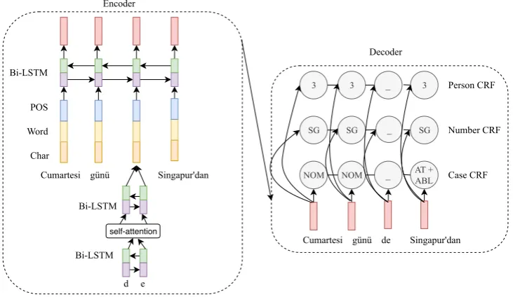
Figure 1: Hierarchical neural model for contextual morphological analysis with independent CRF decoders for each coarse-grained featureF. For the modelMDCRF+POS, POS embeddings are concatenated to the word and char-level representations as depicted above. This model has|F|-1 decoders since POS tagger is run separately as a prior step.MDCRFrefers to the above model without POS embeddings having all|F|decoders.

Token: de Language: <tr> vector 

 t_l:Typological Feature vector Wl

Encoder Decoder

Figure 2: Polyglot model being used for the token “de” in Turkish, denoted by language vector<tr>.

nouns do not have Tense. In order to leverage these linguistic constraints, we incorporate POS information for each token into our shared en-coder. We refer to this variant of the model as

MDCRF+POS, as shown in Figure1.

Since POS tags are not available as input, we first run a separate hierarchical neural CRF tagger for POS alone and use the model predictions as

input to theMDCRF+POS. For each token, we

en-code its predicted POS tag into a continuous repre-sentation and concatenate it with the character and word-level token representations. Finally, these concatenated representations are fed to the word-level bi-LSTM and inference is performed using

|F|-1 decoders, excluding the POS decoder.

Go-ing forward, we use this model architecture for all our experiments unless otherwise noted.

2.2.3 Multi-lingual Transfer

So far, we have described our model architec-ture for a monolingual setting. However, the per-formance of neural models is highly dependent on the availability of large amounts of annotated data, making it challenging to generalize to low-resource languages. Cross-lingual transfer learn-ing attempts to alleviate this challenge by trans-ferring knowledge from high-resource languages.

Prior work (Cotterell and Heigold,2017;Malaviya

et al., 2018; Buys and Botha, 2016) has shown

the benefits of cross-lingual transfer for

morpho-logical tagging. Malaviya et al.(2018) restrict to

transferring from one language, whereasCotterell

and Heigold(2017) show that multi-source

trans-fer performs better than single-source. Inspired by this, we experiment with two approaches for multi-lingual transfer learning.

MULTI-SOURCE: In this method, we augment

the training data from related languages with the

target language data. Similar to Cotterell and

Heigold(2017), we perform a hard clustering of

families such as Germanic and Slavic, we con-struct language clusters from a subset of guages. For instance, the North-Germanic lan-guage cluster comprises of treebanks from Ger-man, Norwegian, Swedish and Danish. Some lan-guages such as Urdu, Tamil are the only represen-tative languages of their respective language fam-ilies in the dataset. For these languages, we create a cluster with the next closest language with re-spect to typology or orthography. For Urdu, we add Hindi because of typological similarity. For other such isolates, we add Turkish because of its extensive agglutination. A total of 24 language clusters were defined based on the literature and with help from a linguist, the details of which can

be seen in the Appendix Section§6.

Given a language cluster, all the training data from each language within it is first concatenated together. Then, for each language we concatenate the language embedding vector with the token rep-resentation in the encoder by adding the language

id<LANG ID>at the beginning and end of each

se-quence. Given a sequencex, the encoder produces

contextualized hidden representation hi for each

tokenxi:

hi=Wencoder(ei, ci, pi, li)

where ei is the word embedding vector, ci is the

character-level representation, pi is the POS

em-bedding and li is the language embedding

vec-tor. This is done to help the model disambiguate languages as often same tokens have different morpho-syntactic description across languages.

For example, the token “ ” is a part of both Hindi

and Marathi vocabulary. In Hindi it denotes a

CONJ whereas in Marathi it is a pronoun with the following description: 3;MASC;PRO;NOM;SG.

POLYGLOT: Languages are often related to

multiple languages along different dimensions. For instance, Swedish is lexically similar to Ger-man, but it is morpho-syntactically closer to En-glish. To enable a model to utilize these relation-ships, we feed explicit typological information to the encoder, drawing inspiration from the

poly-glot model proposed by Tsvetkov et al. (2016).

In this multilingual model, we first concatenate all the training data from the source languages,

simi-lar to theMULTI-SOURCEsetting and computehi

for each token. Then context vectorhi is factored

by the typology feature vectortlto integrate these

manually defined features as follows:

fl = tanh(Wltl+bl)

gl_i =hi⊗flT

where Wl, bl are language-specific parameters

which project the typology vector into a

low-dimentional space. Finally, gl_i computes the

global-context language matrix which is vector-ized into a column vector and fed to the decoder,

as shown in Figure2.

Tsvetkov et al.(2016) derive their typology

vec-tors from the URIEL database (Littell et al.,2017).

We consider a subset of these typology features which are most relevant to the task of morpho-syntactic analysis and obtain 18 Syntax-WALS

features.2 However, we observed that for most

language clusters, these typology feature values within a cluster were not discriminating, which

defeats the purpose of using POLYGLOT for

dis-ambiguating languages across typological dimen-sions. Therefore, we construct custom typologi-cal vector per each language cluster based on the training data global statistics.

For every coarse-grained feature, this con-structed vector contains the proportion of words in the training data that are annotated with that fea-ture. We also experiment with calculating these proportions separately for words for each POS la-bel (N, V, ...). Given the importance of POS, we also include the number of fine-grained POS la-bels that the most frequent coarse-grained features (Gender, Number, Person, Case) can take. This results in bi-gram features such as FEM, N-NOM, N-SG. We remove features which do not occur within a given cluster to avoid sparse

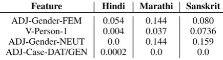
fea-tures. Table1shows a portion of the example

vec-tor constructed for the Indo-Aryan cluster. From the table we can see that, some features such as ADJ-Gender-FEM and V-Person-1 are present in all the three languages within the cluster. Whereas some features such as ADJ-Gender-NEUT is ab-sent from Hindi because Hindi only has two gen-ders which are MASC and FEM.

2

Feature Hindi Marathi Sanskrit

ADJ-Gender-FEM 0.054 0.144 0.080 V-Person-1 0.004 0.037 0.0736 ADJ-Gender-NEUT 0.0 0.144 0.159 ADJ-Case-DAT/GEN 0.0002 0.0 0.0

Table 1: Example of manually constructed typology features for the Indo-Aryan cluster.

Training Regime: For both the multi-lingual transfer methods, we train one model per language cluster and fine-tune this model for each individ-ual language. which saves time and compute for training 107 individual models from scratch. Fur-thermore, since a language cluster can have

mul-tiple high-resource languages, we takemin (5000,

#training data-points) for each language to have

a tractable training time. We up-sample the low-resource languages to match the number of train-ing data-points of the high-resource languages.

3 Contextual Lemmatization

We use the neural model from Malaviya et al.

(2019) for contextual lemmatization. This is a

neural sequence-to-sequence model with hard at-tention, which takes both the inflected form and morphological tag set for a token as input and pro-duces a lemma, both at the character level. The de-coder uses the concatenation of the previous char-acter and the tag set to produce the next charac-ter in the lemma. The lemmatization model is jointly trained with an LSTM-based tagger using jackknifing to reduce exposure bias in training:

Malaviya et al. (2019) report significantly lower

lemmatization results training with gold tags and using predicted tags only at test time. We use their tagger for training and our contextual morpholog-ical analysis models’ predicted tags at evaluation time. This model served as the baseline lemma-tizer for Task 2; we refer readers to the shared task

paper for model details (McCarthy et al.,2019).

4 Experiments

We conduct the following experiments: We com-pare our multi-lingual transfer approach with the

baselinesMalaviya et al.(2018) andCotterell and

Heigold(2017) under the same experimental

set-tings. Next, we compare our approach with the

shared task baseline (McCarthy et al., 2019).

Fi-nally, we analyze the contributions of different components of our proposed method.

Baselines: Cotterell and Heigold(2017) formu-late this task as a sequence prediction problem with the output space being the set of all possi-ble tagsets seen in the training data. Specifically, they construct a neural network based multi-class

classifier where each tagset {N;PL;NOM;FEM}

forms a class. Since the output space is only re-stricted to the tagsets seen in the training data, this method cannot generalize to unseen tagsets. Furthermore, for morphologically rich languages such as Russian or Turkish, the output space of the tagset is huge leading to sparse training data.

(McCarthy et al.,2019) follow a similar approach.

To overcome these drawbacks Malaviya et al.

(2018) consider a feature-wise model which

predicts fine-grained labels for corresponding

coarse categories{POS,Case,...}. Since

morpho-syntactic properties are often correlated, they model these inter-dependencies using a factorial

CRF and define two inter-dependencies: 1) a

pair-wise dependency, which models correlations

be-tween the morpho-syntactic properties within a

to-ken, and 2) atransitiondependency, which models

label correlations across all tokens in a sequence. Although this formulation provides the flexibility to produce any combination of tagsets, this model is computationally expensive to train since the fac-tors model dependencies between all labels of all

coarse-grained features, leading to>20k factors.

Data processing: We use the train/dev/test

split provided in the shared task (McCarthy

et al., 2018).3 Since we model feature-wise

prediction for each coarse-grained feature, our model requires the provided data to be

anno-tated for coarse-grained features. Therefore,

we construct a feature-label dictionary based on

the UM documentation4 to map the individual

fine-grained traits, which are in the UM schema, to their respective coarse-grained categories.

This transforms the tagset{N;PL;NOM;FEM}as

{POS=N;Number=PL;Case=NOM;Gender=FEM}.

We note that usually a token has a subset of the coarse-grained categories, therefore we extend the morphological tagset for each token by adding the remaining features observed in the training set and assigning them a special value “ ” which denotes null.

3

https://github.com/sigmorphon/2019/ tree/master/task2

4_{https://unimorph.github.io/doc/}

Language Model tgt-size=100 tgt-size=1,000

Accuracy F1-Macro F1-Micro Accuracy F1-Macro F1-Micro

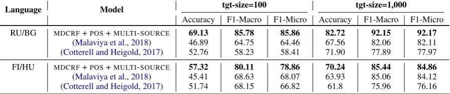
RU/BG MDCRF+POS+MULTI-SOURCE 69.13 85.78 85.86 82.72 92.15 92.17

(Malaviya et al.,2018) 46.89 64.75 64.46 67.56 82.06 82.11 (Cotterell and Heigold,2017) 52.76 58.23 58.41 71.90 77.89 77.97

FI/HU MDCRF+POS+MULTI-SOURCE 57.32 80.11 78.86 70.24 85.44 84.86

(Malaviya et al.,2018) 45.41 68.63 68.07 63.93 85.06 84.12 (Cotterell and Heigold,2017) 51.74 68.15 66.82 61.8 75.96 76.16

Table 2: Comparing our model for bilingual transfer with previous baselines.

Hyper-parameters: We use a hidden size of 200 for each direction of the LSTM with a dropout of 0.5. For the character-level bi-LSTM we use a hidden size of 25. We use 100 dimentional size for word and language embeddings with 64 dimensional POS em-beddings, all randomly initialized. SGD was used as the optimizer with learning rate of 0.015. The

mod-els were trained until convergence. For POLYGLOT,

we project the constructed typology vector into 20 dimension hidden size.

5 Results and Discussion

Table2shows the comparison results of our proposed

approach with the baselines (Malaviya et al.,2018;

Cotterell and Heigold, 2017) using cross-lingual

transfer. HereMDCRF+POS refers to our model

ar-chitecture and MULTI-SOURCE refers to our

multi-lingual transfer approach.Malaviya et al.(2018) and

Cotterell and Heigold (2017) test their approach on

UD v2.1 (Nivre et al.,2017) under two settings: tgt

size = 100 and tgt size = 1000, where tgt size de-notes the number of target language data-points used

during training. Malaviya et al.(2018) transfer from

one related high-resource language. We use the same experimental resources for comparison and for a fair comparison we do not fine-tune on the target

lan-guage. Of the four language pairs tested byMalaviya

et al.(2018), we choose RU/BG and FI/HU for com-parison, where BG and HU are the target languages and RU and FI are the respective transfer languages, since these languages are morphologically challeng-ing. We see that under both settings our approach outperforms the baselines by a significant margin for both the language pairs.

Next, we compare our multi-lingual transfer

ap-proaches MULTI-SOURCE and MULTI-SOURCE +

POLYGLOT in order to decide the model for our

fi-nal submission. We conduct experiments on three

low-resource languages: Marathi (mr-ufal), Sanskrit

(sa-ufal) and Belarusian (be-hse), all of which have

< 400 training data-points. The italicized text

de-notes the treebank used in the experiments. For

mr-ufal and sa-ufal, we transfer from a related

high-resource language of Hindi (hi-hdtb). For be-hse,

we transfer from two related languages, Russian (

ru-gsd) and Ukrainian (uk-iu). However, from Table

3, we see that the performance of the two models

is comparable. Therefore, for our final submission

we use onlyMULTI-SOURCEwhich is much faster to

train than theMULTI-SOURCE+POLYGLOT. We

dis-cuss their comparative performance in greater detail

in Section§5.1.

Model mr-ufal sa-ufal be-hse

MULTI-SOURCE 63.52 / 78.22 42.78 /67.64 77.07/ 82.89 +POLYGLOT 61.18 / 77.42 43.81/ 65.94 76.51 /83.27

Table 3: Multi-lingual comparison results for Marathi (mr-ufal), Sanskrit (sa-ufal) and Belarusian (be-hse) on the validation set.

Finally, we compare our approach with the shared

task baseline. Table5,6in the Appendix shows our

results for all 107 treebanks. We observe that out system achieves an average improvement of +14.70 (accuracy) and +4.63 (F1) over the provided

base-line (McCarthy et al., 2019). We note that for the

shared task submission, we did not use self-attention over the character-level representations. Therefore, we additionally show the results after adding self-attention. We observe that the addition gives an aver-age improvement of +0.60 (accuracy) and +0.30 (F1) over our previous best submission.

5.1 Analysis

Here we analyze the different components of our model in an effort to understand what it is learning.

Why does adding POS help? As discussed

ear-lier (§2), we explicitly add the POS feature in the

form of embeddings into the shared encoder. To

monolingual experiments without concatenating the POS embeddings with the token-level

representa-tions. Table4outlines the ablation results for three

treebanks with varying training size. We observe that

our monolingual modelMDCRFsignificantly

outper-forms the baseline (McCarthy et al.,2019) by +13.72

accuracy and +3.82 F1 (avg). On adding POS, we

further gain +3.56 accuracy and +0.71 F1 overMD

-CRFacross the three treebanks. We note that this

im-provement is more pronounced for the low-medium resource languages of Marathi (+6.12 accuracy) and Ukrainian (+3.57 accuracy).

Model mr-ufal uk-iu hi-hdtb

MDCRF+POS 64.71 / 79.40 84.79 / 92.03 90.46/ 96.69

MDCRF 58.59 / 77.91 81.22 / 91.35 89.45 /96.73

McCarthy et al.(2019) 43.76 / 73.38 63.36 / 87.01 80.96 / 94.14

Table 4: Ablation results for Marathi (mr-ufal), Ukrainian (uk-iu) and Hindi (hi-hdtb) with training size of 373, 5441, 13381 respectively on the validation set.

3 8

72

9

3

54

94

35

67

18 19

2 8

67

8

3

62

77

42

66

14 14

POLAR ITY MOOD POS VER B F OR M TENS E CAS E GENDER PER S ON NUMB ER F INITENES S AS PECT

#

ER

RO

RS

MDCRF MDCRF+POS

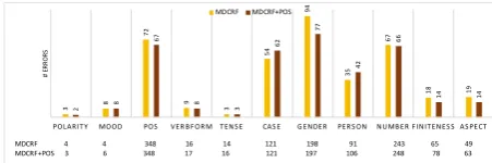
MDCRF 4 4 348 16 14 121 198 91 243 65 49 MDCRF+POS 3 6 348 17 16 121 197 106 248 78 63

Figure 3: Number of errors per coarse-grained feature for Marathi comparing the addition of POS to the en-coder. The rows at the bottom denote the total number of predictions per each feature for both the models.

To understand where the addition of POS helps, we analyse the number of errors made per each coarse-grained feature. For the example of Marathi, POS helped the most in reducing Gender errors

(Fig-ure3). For some word forms, the gender may be

in-ferred from inflectional form alone, but for others,

this information may be insufficient, e.g. “ कमत”

(price.N.FEM.SG.ACC) in Marathi which does not

have the traditional female suffix “ ”. We observe

that this behavior corresponds to POS: verbs and adjectives are more predictable from surface forms alone than nouns. The addition of POS information in the encoder helps the model learn to weigh differ-ent encoded information more heavily when assign-ing gender to different parts of speech. For Ukrainian and Sanskrit, POS information also helped reduce er-rors in Case and Number. More details can be found

in Appendix Section§6.

Tkachenko and Sirts (2018) also model depen-dence on POS with a POS-dependent context vec-tor in the decoder. However, they observe no signif-icant improvement; we hypothesize that incorporat-ing POS information into the shared encoder instead provides the model with a stronger signal.

What is the model learning? One of the major advantages of our model’s use of self-attention is that it enables us to provide insights into what the model

has learned. As seen in Figure 4, we found

evi-dence of the model learning language-specific inflec-tional properties. Both Marathi and Belarusian dis-play morphological inflections predominantly in the form of suffix and the attention maps for both these languages demonstrate the same. For the Marathi ex-ample, the last three characters denote the ergative case and we can see that the attention weights are concentrated on these three characters. Similarly for the Belarusian example, the last two characters de-note the genitive case with plural number and is the focus of the attention. For Indonesian, inflections can be also found as circumfixes where the affix is at-tached at both the beginning and end of the token.

For instance, bothke-and -anaffixes are appended

to form nouns and we can see from Figure4that the

attention is focused both on the prefix and the suf-fix. Interestingly for Indonesian, the model seems to

have also discovered the stem camat, as evidenced

from the attention pattern.

Does time-depth matter for transfer learning?

As discussed earlier, we train one model per lan-guage cluster for multi-lingual transfer learning. We

compare different clusters to see if time-depth of

the languages within a cluster affects the extent of

transfer. Time depth is the period of time that has

elapsed since all languages in the group were a sin-gle language (in other words, the time since

di-vergence). We consider the following three

clus-ters: Hindi-Marathi-Sanskrit (Indo-Aryan), Russian-Ukrainian-Belarusian (Slavic) and Arabic-Hebrew-Amharic-Akkadian (Semitic). These three clusters were chosen because the languages in them became separate languages at varying time-depths. For in-stance, in the Semitic cluster the languages diverged roughly 5000 years ago, whereas for the Slavic

clus-ter the time-depth is<1000 years. Therefore, we

ex-pect transfer to help more for languages where the

time-depth is more recent. In Figure 5, we

mono-न

◌ो

क

र

◌ा

न

◌े

न ◌ो क र ◌ा न ◌े

नोकराने = नोकर + ◌ान ◌े ‘servant’ servant.N.MASC.SG by.ERG

(a) Marathi

kecamatan = ke + camat + an ‘district office’ NOM district.head.N NOM

(b) Indonesian

выпадкаў = выпадак + аў ‘of occassions’ occassion.MASC.N.INAN GEN.PL

(c) Belarusian

Figure 4: Character-level attention maps for three typologically different languages. Marathi and Belarusian dis-play morphological inflections pre-dominantly as suffix. Indonesian disdis-plays inflections in the form of prefix, suffix and circumfix where the affix is found both at the beginning and end of a token.

lingual modelMDCRF+POSand we see that transfer

helps most for the Slavic cluster by +2.9 accuracy. For the Indo-Aryan cluster it helps by +0.32 accu-racy and for the Semitic cluster we observe a slight negative effect with transfer (-0.0176 accuracy). This

supports our hypothesis that time-depth does affect

the extent of transfer learning with language clusters

having lowertime-depthsbenefiting the most.

One particular advantage that the Slavic cluster has over both the Indo-Aryan and Semitic clusters is the similarity of script. Russian, Belarusian, and Ukrainian use variants of the same script; Hindi, Sanskrit, and Marathi do, as well, but the Semitic languages all use different scripts. This is also at-tributed to the shallower time-depths of the Slavic and Indo-Aryan clusters. Therefore, as suggested by the anonymous reviewers, we add Czech and Polish to the Slavic cluster and see to what extent the scripts are confusing the model. Czech and Polish use dif-ferent script as compared to Russian, Belarusian, and

Ukrainian. We observe thatMULTI-SOURCE model

like before, achieves similar improvements over the monolingual models for Belarusian (+8.17 accuracy) and Ukrainian (+1.2 accuracy). However, a slight de-crease is observed for Russian ( -0.45 accuracy). This

suggests that theMULTI-SOURCEmodel is robust to

scriptal changes and benefits the low-resource guages by learning from typologically similar lan-guages, more so for language clusters with shallow time-depths.

0.23 ₀ 0.75

6.89

0.82 0.99 0.36

1.85

-0.17

-3.12 0.2

Absolute gain

-4 -2 0 2 4 6 8

mr_ufal sa_ufal hi_hdtb be_hse ru_gsd uk_iuar_padt ar_pud he_htb

ak_pisandub amh_att

Figure 5: Absolute gain of multi-lingual transfer over monolingual models. Blue denotes the Indo-Aryan

cluster, pink theSlavic, and yellow theSemitic.

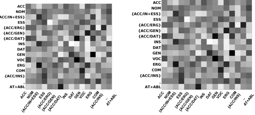
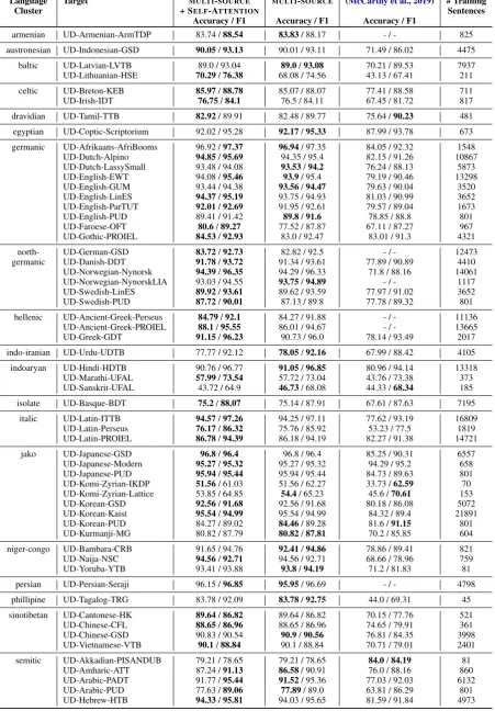
Why didPOLYGLOTnot help further? We

hy-pothesize that one reason why POLYGLOT did not

help over MULTI-SOURCE is because the language

embedding vector probably learns the same typo-logical information which the typology vector en-codes. Hence, the typological vector doesn’t seem to add any new information. As evidence, we look at the transition weights learned in both the models; as

shown in Figure7, we see that the transition weights

learned for the Case feature are very similar for both

MULTI-SOURCEand MULTI-SOURCE+POLYGLOT.

In the future, we plan to explore the contextual

pa-rameter generation method (Platanios et al., 2018)

ACC NOM

{ACC/IN+ESS} ESS

{ACC/ERG} {ACC/GEN}{ACC/DA

T} INS DA T

GENVOC ERG COM

{ACC/INS} _

AT+ABL

ACC NOM

{ACC/IN+ESS} ESS

{ACC/ERG} {ACC/GEN}{ACC/DA

T} INS DA T

GENVOC ERG COM

{ACC/INS} _

AT+ABL

Figure 6: Transition weights for the Case feature for Hindi across MULTI-SOURCE (left) and MULTI-SOURCE+

POLYGLOT(right) models trained with Hindi (hi-hdtb), Marathi (mr-ufal) and Sanskrit (sa-ufal).

5.2 Error Analysis

In this section, we analyze the major error categories

for the MULTI-SOURCE model for the Indo-Aryan

cluster. We observe that Gender, Case, Number, Per-son features account for the most number of errors (65% for Marathi, 49% for Sanskrit). One reason for this is the non-overlapping output label space across the languages within a cluster. For instance, in the Indo-Aryan cluster, Hindi is a high-resource

language (> 13k training sentences) with Marathi

(373) and Sanskrit (184) being the low-resource lan-guages. We observe that the label space for Case, Gender, Number overlap the least among the three

languages. Marathi and Sanskrit have three

gen-ders: NEUT, FEM, MASC whereas Hindi only has

FEM, MASC. Furthermore, only two Hindi Case

la-bels (ACC, NOM) overlap with Marathi and Sanskrit

because in Hindi the labels often have alternatives

such as ACC/ERG, ACC/DAT. These differences in

the output space negatively affect the transfer. For the Slavic cluster, we observe that almost all the fea-ture labels overlap nicely for the languages therein, which is probably another reason why we see a gain

of +6.89 for Belarusian in Figure5and only +0.32

increase for Marathi.

We also note that for some languages such as Be-larusian and Russian, the POS errors increased by

25.3% and 4.4% respectively for the MDCRF+POS

model. This suggests that decoupling POS feature from the other feature decoders harmed the model. In

future, we plan to improve the MDCRF+POS model

by jointly training POS decoder with the other

fea-ture decoders which use the latent representation of POS in an end-to-end fashion.

6 Conclusion and Future Work

We implement a hierarchical neural model with in-dependent decoders for each coarse-grained morpho-logical feature and show that incorporating POS in-formation in the shared encoder helps improve pre-diction for other features. Furthermore, our multi-lingual transfer methods not only help improve re-sults for related languages but also eliminate the need of training individual models for each dataset from scratch. In future, we plan to explore the use of pre-trained multi-lingual word embeddings such as

BERT (Devlin et al.,2019), in our encoder.

Acknowledgement

We are thankful to the anonymous reviewers for their valuable suggestions.

References

Jan Buys and Jan A. Botha. 2016. Cross-lingual mor-phological tagging for low-resource languages. In

Proc. of ACL, pages 1954–1964.

Ryan Cotterell and Georg Heigold. 2017. Cross-lingual character-level neural morphological tag-ging. InProc. of EMNLP, pages 748–759.

Onur G¨ung¨or, Suzan ¨Usk¨udarlı, and Tunga G¨ung¨or. 2018. Improving named entity recognition by jointly learning to disambiguate morphological tags.

arXiv preprint arXiv:1807.06683.

Jan Hajic and Barbora Hladk´a. 1998. Tagging inlective languages: Prediction of morphological categories for a rich structured tagset. In Proc. of ACL, vol-ume 1.

Georg Heigold, Guenter Neumann, and Josef van Gen-abith. 2017. An extensive empirical evaluation of character-based morphological tagging for 14 lan-guages. InProc. of EACL, pages 505–513.

Daniel Kondratyuk. 2019. 75 languages, 1 model: Parsing universal dependencies universally. arXiv preprint arXiv:1904.02099.

Guillaume Lample, Miguel Ballesteros, Sandeep Sub-ramanian, Kazuya Kawakami, and Chris Dyer. 2016. Neural architectures for named entity recognition. InProc. of NAACL, pages 260–270.

Patrick Littell, David R Mortensen, Ke Lin, Kather-ine Kairis, Carlisle Turner, and Lori Levin. 2017. Uriel and lang2vec: Representing languages as ty-pological, geographical, and phylogenetic vectors. InProc. of EACL, volume 2, pages 8–14.

Xuezhe Ma and Eduard Hovy. 2016. End-to-end sequence labeling via bi-directional LSTM-CNNs-CRF. InProc. of ACL, pages 1064–1074.

Chaitanya Malaviya, Matthew R. Gormley, and Gra-ham Neubig. 2018. Neural factor graph models for cross-lingual morphological tagging. In Proc. of ACL, pages 2653–2663.

Chaitanya Malaviya, Shijie Wu, and Ryan Cot-terell. 2019. A simple joint model for improved contextual neural lemmatization. arXiv preprint arXiv:1904.02306v2.

Arya D. McCarthy, Miikka Silfverberg, Ryan Cotterell, Mans Hulden, and David Yarowsky. 2018. Marrying Universal Dependencies and Universal Morphology. InProceedings of the Second Workshop on Univer-sal Dependencies (UDW 2018), pages 91–101.

Arya D. McCarthy, Ekaterina Vylomova, Shijie Wu, Chaitanya Malaviya, Lawrence Wolf-Sonkin, Gar-rett Nicolai, Christo Kirov, Miikka Silfverberg, Se-bastian Mielke, Jeffrey Heinz, Ryan Cotterell, and Mans Hulden. 2019. The SIGMORPHON 2019 shared task: Crosslinguality and context in

morphol-ogy. In Proceedings of the 16th SIGMORPHON

Workshop on Computational Research in Phonetics, Phonology, and Morphology.

Thomas M¨uller and Hinrich Schuetze. 2015. Robust morphological tagging with word representations. InProc. of NAACL, pages 526–536.

Joakim Nivre, ˇZeljko Agi´c, Lars Ahrenberg, Lene An-tonsen, Maria Jesus Aranzabe, Masayuki Asahara, Luma Ateyah, Mohammed Attia, Aitziber Atutxa, Liesbeth Augustinus, et al. 2017. Universal depen-dencies 2.1.

Kemal Oflazer and Ilker Kuru¨oz. 1994. Tagging and morphological disambiguation of turkish text. In

Proc. of ANLP, pages 144–149.

Emmanouil Antonios Platanios, Mrinmaya Sachan, Graham Neubig, and Tom Mitchell. 2018. Contex-tual parameter generation for universal neural ma-chine translation. InProc. of EMNLP, pages 425– 435.

Emma Strubell, Patrick Verga, Daniel Andor, David Weiss, and Andrew McCallum. 2018. Linguistically-informed self-attention for seman-tic role labeling. In Proc. of EMNLP, pages 5027–5038.

Alexander Tkachenko and Kairit Sirts. 2018. Modeling composite labels for neural morphological tagging.

arXiv preprint arXiv:1810.08815.

Yulia Tsvetkov, Sunayana Sitaram, Manaal Faruqui, Guillaume Lample, Patrick Littell, David Mortensen, Alan W. Black, Lori Levin, and Chris Dyer. 2016. Polyglot neural language models: A case study in cross-lingual phonetic representation learning. InProc. of NAACL, pages 1357–1366.

Ashish Vaswani, Noam Shazeer, Niki Parmar, Jakob Uszkoreit, Llion Jones, Aidan N Gomez, Łukasz Kaiser, and Illia Polosukhin. 2017. Attention is all you need. InProc. of NIPS, pages 5998–6008.

Ekaterina Vylomova, Trevor Cohn, Xuanli He, and Gholamreza Haffari. 2017. Word representation models for morphologically rich languages in neu-ral machine translation. InProceedings of the First Workshop on Subword and Character Level Models in NLP, pages 103–108.

Appendix

Comprehensive Results

Table 5 and 6 document the comprehensive results

of our submissions. MULTI-SOURCE was our

pre-vious submission to the shared task. We conducted additional experimentas with the addition of

self-attention and also report the results for MULTI

-SOURCE+SELF-ATTENTION. We report both the

ac-curacy and F1 metric.

Language Clusters

We train one model per language cluster for the multi-lingual transfer learning. Each language clus-ter was constructed based on the typological

similar-ity of the languages therein. Table5,6show the

lan-guage clusters.

Analysis

In order to understand where the addition of POS helps, we plot the number of errors per each

coarse-grained feature for three languages in Figure7. For

Sanskrit and Ukrainian we see that POS generally helps reduce the errors predominantly for the fea-tures: Case, Gender, Number. For Belarusian, we did not observe a clear trend since the POS accuracy

Language Target MULTI-SOURCE MULTI-SOURCE (McCarthy et al.,2019) # Training

Cluster + SELF-ATTENTION Sentences

Accuracy / F1 Accuracy / F1 Accuracy / F1

armenian UD-Armenian-ArmTDP 83.74 /88.54 83.83/ 88.17 - / - 825

austronesian UD-Indonesian-GSD 90.05/93.13 90.01 / 93.11 71.49 / 86.02 4475

baltic UD-Latvian-LVTB 89.0 / 93.04 89.0/93.08 70.21 / 89.53 7937

UD-Lithuanian-HSE 70.29/76.38 68.08 / 74.56 43.13 / 67.41 211

celtic UD-Breton-KEB 85.97/88.78 85.07 / 88.07 77.41 / 88.58 711

UD-Irish-IDT 76.75/84.1 76.5 / 84.11 67.45 / 81.72 817

dravidian UD-Tamil-TTB 82.92/ 89.91 82.48 / 89.77 75.64 /90.23 481

egyptian UD-Coptic-Scriptorium 92.02 / 95.28 92.17/95.33 87.99 / 93.78 673

germanic UD-Afrikaans-AfriBooms 96.92 /97.37 96.94/ 97.35 84.05 / 92.32 1548

UD-Dutch-Alpino 94.85/95.69 94.35 / 95.4 82.15 / 91.26 10867

UD-Dutch-LassySmall 93.48 / 94.08 93.53/94.2 76.24 / 88.13 5873

UD-English-EWT 94.08 /95.46 93.9/ 95.4 79.19 / 90.46 13298

UD-English-GUM 93.44 / 94.38 93.56/94.47 79.63 / 90.04 3520

UD-English-LinES 94.37/95.19 93.75 / 94.93 81.03 / 90.99 3652

UD-English-ParTUT 92.01/92.69 91.95 / 92.61 79.57 / 89.04 1673

UD-English-PUD 89.41 / 91.42 89.8/91.6 78.85 / 88.8 801

UD-Faroese-OFT 80.6/89.27 77.52 / 87.87 67.11 / 87.27 967

UD-Gothic-PROIEL 84.53/92.93 83.0 / 92.47 83.01 / 91.3 4321

north- UD-German-GSD 83.72/92.73 82.82 / 92.5 - / - 12473

germanic UD-Danish-DDT 91.78/93.72 91.34 / 93.61 77.89 / 90.89 4410

UD-Norwegian-Nynorsk 94.39/96.35 94.29 / 96.33 71.8 / 88.16 14061

UD-Norwegian-NynorskLIA 93.03 / 94.55 93.75/94.89 - / - 1117

UD-Swedish-LinES 89.92/93.61 89.62 / 93.59 77.97 / 91.02 3652

UD-Swedish-PUD 87.72/90.01 87.13 / 89.8 77.78 / 89.32 801

hellenic UD-Ancient-Greek-Perseus 84.79/92.1 84.27 / 91.88 - / - 11136

UD-Ancient-Greek-PROIEL 88.1/95.55 86.01 / 94.67 - / - 13665

UD-Greek-GDT 91.15/96.23 90.73 / 96.0 78.14 / 93.49 2017

indo-iranian UD-Urdu-UDTB 77.77 / 92.12 78.05/92.16 67.99 / 88.42 4105

indoaryan UD-Hindi-HDTB 90.76 / 96.77 91.05/96.85 80.96 / 94.14 13318

UD-Marathi-UFAL 57.99/73.54 57.72 / 73.04 43.76 / 73.38 373

UD-Sanskrit-UFAL 43.72 / 64.9 46.73/ 68.08 44.33 /68.34 185

isolate UD-Basque-BDT 75.2/88.07 75.14 / 87.91 67.61 / 87.63 7195

italic UD-Latin-ITTB 94.57/97.26 94.25 / 97.11 77.62 / 93.19 16809

UD-Latin-Perseus 76.17/86.32 75.76 / 85.92 53.23 / 77.5 1819

UD-Latin-PROIEL 86.78/94.39 86.18 / 94.19 82.27 / 91.38 14721

jako UD-Japanese-GSD 96.8/96.4 96.8 / 96.4 85.25 / 90.31 6557

UD-Japanese-Modern 95.27/95.32 95.27 / 95.32 94.29 / 95.2 658

UD-Japanese-PUD 95.94/95.44 95.94 / 95.44 84.73 / 89.63 801

UD-Komi-Zyrian-IKDP 51.56/ 61.03 51.56 / 62.27 33.73 /62.59 70

UD-Komi-Zyrian-Lattice 53.85 / 64.85 54.4/ 65.23 45.6 /70.61 153

UD-Korean-GSD 92.56/91.68 92.56 / 91.68 80.18 / 86.08 5072

UD-Korean-Kaist 95.54/94.99 95.54 / 94.99 84.32 / 89.4 21891

UD-Korean-PUD 84.27 / 89.02 84.46/ 89.28 81.6 /91.15 801

UD-Kurmanji-MG 80.82 / 87.79 80.82/87.81 70.2 / 85.85 604

niger-congo UD-Bambara-CRB 91.65 / 94.76 92.41/94.86 78.86 / 89.41 821

UD-Naija-NSC 94.56/92.71 94.56 / 92.71 68.66 / 78.96 759

UD-Yoruba-YTB 93.41 / 93.88 93.8/94.19 71.2 / 81.83 81

persian UD-Persian-Seraji 96.15 /96.85 95.95/ 96.69 - / - 4798

phillipine UD-Tagalog-TRG 83.78 / 92.09 83.78/92.75 44.0 / 69.31 45

sinotibetan UD-Cantonese-HK 89.64/86.82 89.64 / 86.82 70.15 / 77.76 521

UD-Chinese-CFL 88.65/86.96 88.65 / 86.96 74.65 / 79.91 361

UD-Chinese-GSD 90.83 / 90.54 90.9/90.56 76.81 / 84.35 3998

UD-Vietnamese-VTB 90.1/88.84 90.1 / 88.84 70.71 / 79.01 2401

semitic UD-Akkadian-PISANDUB 79.21 / 78.65 79.21 / 78.65 84.0/84.19 81

UD-Amharic-ATT 87.24 /91.13 86.58/ 90.91 76.0 / 88.16 860

UD-Arabic-PADT 91.77 /95.44 91.52/ 95.36 77.03 / 92.03 6132

UD-Arabic-PUD 77.63 /89.06 77.89/ 89.0 63.81 / 86.29 801

UD-Hebrew-HTB 94.33/95.81 94.03 / 95.65 81.59 / 91.84 4973

Cluster Target MULTI-SOURCE MULTI-SOURCE (McCarthy et al.,2019) # Training

+ SELF-ATTENTION Sentences

Accuracy / F1 Accuracy / F1 Accuracy / F1

turkic UD-Turkish-IMST 85.68/90.64 85.02 / 90.43 62.04 / 85.33 4509

UD-Turkish-PUD 79.78/90.88 79.33 / 90.54 66.92 / 88.05 801

romance UD-Catalan-AnCora textbf96.68 /98.26 96.63 / 98.24 85.77 / 95.7 13343

UD-French-GSD 96.19 /97.51 95.76/ 97.32 84.44 / 94.81 13074

UD-French-ParTUT 93.04 / 96.05 93.04/96.12 81.32 / 92.08 817

UD-French-Sequoia 95.08/ 96.95 94.96 /96.96 82.64 / 93.42 2480

UD-French-Spoken 96.05/96.08 96.05 / 96.08 94.57 / 94.85 2229

UD-Galician-CTG 96.65 / 96.31 96.66/96.32 87.23 / 91.81 3195

UD-Galician-TreeGal 89.69/ 93.2 89.3 /93.25 76.85 / 90.05 801

UD-Italian-ISDT 95.91 / 97.24 95.96/97.27 83.62 / 94.34 11334

UD-Italian-ParTUT 95.0/ 96.39 94.87 / 96.39 84.03 / 93.42 1673

UD-Italian-PoSTWITA 92.13/93.13 92.03 / 93.02 70.23 / 88.18 5371

UD-Italian-PUD 87.55/ 92.4 87.38 /92.46 80.89 /92.66 801

UD-Portuguese-Bosque 92.28/95.57 92.06 / 95.5 63.14 / 86.12 7493

UD-Portuguese-GSD 97.33/97.54 97.33 / 97.54 - / - 9663

UD-Romanian-Nonstandard 91.13/95.33 91.07 / 95.29 74.31 / 91.5 8056

UD-Romanian-RRT 94.67 / 96.58 94.82/96.63 81.45 / 93.96 7620

UD-Spanish-AnCora 96.97/98.25 96.86 / 98.22 84.27 / 95.3 14145

UD-Spanish-GSD 94.05 / 97.08 94.07/97.1 - / - 12811

slavic UD-Belarusian-HSE 79.63/85.37 77.28 / 84.11 54.99 / 79.07 315

UD-Bulgarian-BTB 94.22/96.44 93.99 / 96.37 79.75 / 93.91 8911

UD-Buryat-BDT 78.85/81.24 75.96 / 78.66 63.26 / 78.53 742

UD-Old-Church-Slavonic-PROIEL 87.22/94.13 86.94 / 94.03 82.86 / 90.34 5070

UD-Russian-GSD 84.26/91.91 83.25 / 91.55 64.42 / 88.77 4025

UD-Russian-PUD 76.77 /87.55 77.25/ 87.49 63.15 / 85.52 801

UD-Russian-SynTagRus 91.65 / 95.96 92.74/96.5 73.9 / 92.84 49512

UD-Russian-Taiga 74.14 / 80.23 75.24/81.25 52.99 / 78.71 1412

UD-Ukrainian-IU 86.02/92.41 85.33 / 92.2 63.36 / 87.01 5441

UD-Upper-Sorbian-UFAL 74.04/82.45 70.12 / 81.21 55.66 / 78.3 517

ugric UD-Estonian-EDT 87.71 / 94.58 88.47/94.93 74.56 / 91.71 24579

UD-Finnish-FTB 83.24 / 90.38 83.63/90.7 73.16 / 89.51 14979

UD-Finnish-PUD 77.05 / 86.33 77.49/86.77 71.65 /88.87 801

UD-Hungarian-Szeged 80.57/90.88 79.16 / 90.13 63.72 / 87.29 1441

UD-North-Sami-Giella 84.35/88.8 83.78 / 88.65 67.04 / 85.6 2498

UD-Norwegian-Bokmaal 94.97/96.68 94.58 / 96.51 81.44 / 93.19 16037

UD-Swedish-Talbanken 93.94/96.01 93.64 / 95.9 - / - 4821

UD-Finnish-TDT 86.51/92.63 85.55 / 92.2 75.13 / 90.92 12109

westslavic UD-Croatian-SET 87.23/94.04 86.88 / 93.91 72.71 / 90.99 7112

UD-Czech-CAC 90.66 / 96.72 91.38/96.99 77.15 / 93.92 19768

UD-Czech-CLTT 91.29/ 96.15 91.07 /96.22 73.92 / 92.37 901

UD-Czech-FicTree 90.05 / 95.42 90.0/95.49 68.28 / 90.37 10209

UD-Czech-PDT 89.78/96.37 54.13 / 73.56 76.69 / 94.28 70331

UD-Czech-PUD 75.65 / 88.19 77.72/89.37 59.54 / 85.5 801

UD-Polish-LFG 87.76 /93.7 87.81/ 93.65 - / - 13797

UD-Polish-SZ 82.27/91.38 81.01 / 90.88 65.58 / 88.29 6582

UD-Serbian-SET 91.89/95.46 91.35 / 95.29 75.73 / 91.19 3113

UD-Slovak-SNK 85.59/93.12 84.99 / 92.83 64.24 / 88.16 8484

UD-Slovenian-SSJ 89.05/94.03 87.92 / 93.55 73.73 / 89.95 6401

UD-Slovenian-SST 85.13 /90.16 85.51/ 90.02 73.4 / 84.74 2551

0

17

71

7

30

98

0

81

18 21

75

67

21

38

0

29

89

6

39

117

3

85

15

35

75

52

35

48

POLA I RT Y M OOD POS V E RBF ORM T E NS E CA S E COM PA RI S ON GE ND E R PE RS ON V OI CE A NI M A CY NUM BE R F I NI T E NE S S A S PE CT

#

ER

RO

RS

MDCRF MRCRF+POS

MDCRF 9 49 590 1 44 366 3 340 27 73 247 423 66 73 MDCRF+POS 9 69 590 6 74 346 3 330 45 95 244 410 87 95

(a) Belarusian (be-hse)

3

90

585

27 94

1018

24 ₀

640

64 ₃₀

622

416

95

290

2

104

615

23 101

856

20 2

568

67 ₂₅

603

330

111

288

POLA RI T Y M OOD POS V E RBF ORM T E NS E CA S E COM PA RI S ON V A LE NCY GE ND E R PE RS ON V OI CE A NI M A CY NUM BE R F I NI T E NE S S A S PE CT

#

ER

RO

RS

MDCRF MDCRF+POS

MDCRF 128 995 9182 140 987 6467 58 46 5004 805 103 3619 6202 1216 1333 MDCRF+POS 129 1053 9185 148 1044 6435 70 46 4957 855 113 3602 6177 1280 1427

(b) Ukrainian (uk-iu)

1

8

68

1

19 19

61 66

8

22

40

6

2

1

9

60

1

19 23

51

62

9

26

37

8

2

POLA RI T Y M OOD POS POLI T E NE S S V E RBF ORM T E NS E CA S E GE ND E R PE RS ON V OI CE NUM BE R F I NI T E NE S S A S PE CT

#

ER

RO

RS

MDCRF MDCRF+POS

MDCRF 6 12 178 0 1 9 102 99 15 14 141 12 7 MDCRF+POS 6 21 178 0 9 18 106 105 22 31 134 22 7

(c) Sanskrit (sa-ufal)