Efficient Language Modeling with Automatic Relevance Determination in Recurrent Neural Networks

40

Efficient Language Modeling with Automatic Relevance Determination in

Recurrent Neural Networks

Maxim Kodryan∗

Moscow State University Moscow, Russia

[email protected]

Artem Grachev∗

Samsung R&D Institute, National Research University

Higher School of Economics Moscow, Russia

[email protected]

Dmitry Ignatov

National Research University Higher School of Economics

Moscow, Russia

Dmitry Vetrov

Samsung AI Center, National Research University

Higher School of Economics Moscow, Russia

Abstract

Reduction of the number of parameters is one of the most important goals in Deep Learn-ing. In this article we propose an adaptation of Doubly Stochastic Variational Inference for Automatic Relevance Determination (DSVI-ARD) for neural networks compression. We find this method to be especially useful in lan-guage modeling tasks, where large number of parameters in the input and output layers is of-ten excessive. We also show that DSVI-ARD can be applied together with encoder-decoder weight tying allowing to achieve even better sparsity and performance. Our experiments demonstrate that more than 90% of the weights in both encoder and decoder layers can be re-moved with a minimal quality loss.

1 Introduction

The problem of neural networks compression has recently gained more interest as the number of pa-rameters (and hence memory size) of modern neu-ral networks increased drastically. Moreover, only a few weights prove to be relevant for prediction while the majority are de facto redundant (Han et al.,2015).

In this paper we suggest an adaptation of a Bayesian approach called Automatic Relevance Determination (ARD) for neural networks com-pression in language modeling tasks, where the first and the last linear layers often have enormous

∗

These two authors contributed equally; the ordering of their names was chosen arbitrarily. The work was done when the first author was an intern at the Samsung R&D Institute.

size. We derive theDoubly Stochastic Variational Inference (DSVI) algorithm for non-iid (not in-dependent and identically distributed) objects, a common case in language modeling, and use it to perform optimization of our models.

Furthermore, we extend this approach so that it could be applied together with the weight ty-ing technique (Press and Wolf,2017;Inan et al.,

2016), i.e., using the same set of parameters for both weight matrices of the first and the last lay-ers, which has been proved highly efficient.

2 Related works

Most of the works on neural networks com-pression can be roughly divided into two cate-gories: those dealing with matrix decomposition approaches (Lu et al.,2016;Arjovsky et al.,2016;

Tjandra et al., 2017; Grachev et al., 2019) and those that leverage pruning techniques (Han et al.,

2015;Narang et al.,2017). From this point of view methods based on Bayesian techniques (Louizos et al.,2017;Molchanov et al.,2017) can be con-sidered as a more mathematically justified version of pruning.

poorly theoretically justified (Hron et al., 2018), whereas ARD does not encounter these issues while maintaining similar efficacy (Kharitonov et al.,2018).

At last, as far as we are concerned, combin-ing DSVI-ARD (or other Bayesian prunncombin-ing tech-niques) with weight tying has not been considered previously.

3 Language modeling with neural

networks

The language modeling problem is one of the im-portant classical NLP problems and has various applications such as machine translation and text classification.

This problem is usually formulated as

probabilistic prediction of a word sequence

(w1, . . . , wT) = (wi)Ti=1as follows:

P(wi)Ti=1

=PwT|(wi)Ti=1−1

P(wi)Ti=1−1

=

=

T

Y

t=1

Pwt|(wi)ti=1−1

≈

T

Y

t=1

Pwt|(wi)it=−1t−T0

(1)

The last equation in (1) is approximated as it is almost always impossible to calculate this expres-sion exactly for a sequence of words of arbitrary length. Therefore, the calculation is performed only within a context of a fixed sizeT0.

Nowadays, approaches that perform the approx-imation for whole words involve different vari-ations of RNNs (Bengio et al., 2003; Mikolov,

2012) such as LSTM or GRU (Hochreiter and Schmidhuber, 1997;Cho et al., 2014). In word-level models the input layer maps words from the vocabulary Vto some vector representation, and vice versa for the output layer: from a vector to a distribution over words in the vocabulary. It leads to sizes of these layers being proportional to the vocabulary size|_V|which is tens of thousands in a typical use case.

Assume using LSTM cells as recurrent units. We can compute the total number of parameters in a network via the following formula:

ntotal = 8LD2+ 2|V|D, (2)

whereLis the number of recurrent hidden layers, andDis the hidden layers size (for simplicity we let all hidden layers be of the same size). Various

designs (Bengio and Senecal, 2003; Chen et al.,

2016) have been proposed to reduce it, but still in word-level language modeling tasks with a signif-icantly large vocabulary size the second term in the sum (2) makes the largest contribution. Some-times the softmax (decoder) layer can solely oc-cupy up to a third of the whole network memory space.

The following section describes the technique that performs efficient reduction of parameters in linear layers. This technique can be applied to the decoder layer of RNN (or to both decoder and encoder layers in tied-weight setting) providing the overall network compression with a negligible drop in quality.

4 DSVI-ARD

In this section we describe how the Dou-bly Stochastic Variational Inference algorithm for Automatic Relevance Determination (DSVI-ARD) originally proposed in (Titsias and L´azaro-Gredilla, 2014) can be adopted for solving mul-ticlass classification task and, thus, leveraged in neural networks training for compressing their dense layers (in particular, decoder layers in RNNs).

4.1 Automatic Relevance Determination

We formulate the multiclass classification problem in a Bayesian framework that can provide a useful tool for feature selection — the so-called Auto-matic Relevance Determination (ARD).1

Consider a discriminative probabilistic model given a training dataset(X, Y) = {(xn, yn)}Nn=1

ofN independent objects:

p(W, Y |X,Λ) =p(W |Λ)

N

Y

n=1

p(yn|W,xn) =

=

K

Y

i=1

D

Y

j=1

N (wij |0, λij) N

Y

n=1

Softmax (Wxn)yn

(3)

Here xn ∈ RD is the feature vector of then-th object, yn ∈ {1, . . . , K} is the label of the n

-th object’s class, W ∈ _RK×D _{is the matrix of}

model parameters and Λ ∈ _RK×D _{is the matrix}

of hyperparameters defining the prior distribution

p(W |Λ)over parametersW.

1_{Here we consider linear classification for simplicity,}

The prior distribution p(W | Λ)is considered to be element-wise factorized Gaussian over each elementwij (zero mean and tunable varianceλij).

The likelihood function p(yn|W,xn) is theyn

-th element of -the softmax vector of linear logits

Wxn. Such a likelihood function is quite typical

in classification tasks and can be encountered in multivariate Logistic Regression.

The two goals of the subsequent Bayesian infer-ence are, first, obtaining posterior distribution over the model parameters conditioned on the training dataset p(W |X, Y,Λ), which can be leveraged in prediction on the test set, and, second, opti-mal model selection, i.e., hyperparameters tuning. Both problems can be solved simultaneously by maximizing the Evidence Lower Bound (ELBO):

L(q,Λ) =EW∼q(W)[logp(Y |W, X)]−

−KL(q(W)kp(W |Λ)). (4)

ELBO is a function of two variables: an ar-bitrary variational distribution over parameters

q(W) and model hyperparameters Λ, and can be decomposed into two parts: the data term EW∼q(W)[logp(Y |W, X)]and the negative

KL-divergence between the variational approximation

q(W) and the prior distribution p(W | Λ) (KL-term) −KL(q(W)kp(W |Λ)). We further show that maximization of ELBO with respect to both

qandΛsolves the model selection problem while also fittingqto the posterior.

ELBO has several useful properties such as L(q,Λ)≤logp(Y |X,Λ),∀q,Λ(bounds the

ev-idence logarithm logp(Y | X,Λ) from

be-low) and L(q,Λ) = logp(Y |X,Λ) if and only if q(W) =p(W |X, Y,Λ), so maximization of ELBO with respect toq for fixedΛ is equivalent to fittingqto the posteriorp(W |X, Y,Λ), hence solving the first of the mentioned Bayesian infer-ence problems.

Maximization of the evidence p(Y | X,Λ)

with respect to hyperparametersΛis a well-known Bayesian model selection method, also known as empirical Bayes estimation (Carlin and Louis,

1997). A model with the highest evidence is con-sidered to be “the best” in terms of both data fit and model complexity. Evidence maximization can be performed via ELBO maximization as

max

Λ logp(Y |X,Λ) = maxq,Λ L(q,Λ). (5)

Finally, this double maximization procedure, as

we have shown above, handles the model selection problem while also fittingqto the posterior.

From the view of the ELBO functional it is clear that only the KL-term KL(q(W)kp(W |Λ) de-pends on Λ, hence maximization of ELBO with respect toΛ is equivalent to minimization of the KL-term with respect toΛ.

Now we restrict the variational distributionq to the factorized Gaussian:

q(W |µ,σ) =

K

Y

i=1

D

Y

j=1

N(wij |µij, σ2ij), (6)

whereµ,σ ∈ _RK×D _{are thevariational}

parame-ters.

This way ELBO maximization (or equivalently, KL-term minimization) with respect toΛ can be performed analytically with the solution at

λ∗_ij =µ2_ij+σ_ij2. (7)

After substituting Λ∗ from (7) into the ELBO equation (4) and taking into account the varia-tional family restriction (6) we can rewrite the maximization problem (5) as follows:

EW∼q(W|µ,σ)[logp(Y |W, X)] +

+ 1 2

K

X

i=1

D

X

j=1

log σ

2

ij

µ2

ij+σ2ij

−→max µ,σ

(8)

This equation (8) is the final form of the ARD ELBO maximization problem. We can see that the first term (data term) induces the variational parameters to describe the observed data well by sharpening the variational distribution at the maxi-mum likelihood point, while the second term (KL-term) makes irrelevant parameters shrink. The mutual maximization of both terms leads to a sparse solution (in the limit), at which all redun-dant features are zeroed. The following subsec-tions describe how it can be performed in practice, especially in application to recurrent neural net-works.

4.2 DSVI

and a set of “proto-weights” for each object in the mini-batch m∼ N(0, I),m∈RK×D, which are used to obtain stochastic gradients of the log-likelihood with respect to the varia-tional parameters via the reparametrization trick (RT) (Kingma et al., 2015). DSVI does not de-pend on a specific form of the log-likelihood func-tion logp(y | W, x), but only requires its gradi-ent∇Wlogp(y |W, x), so the same procedure is

applicable for different models with differentiable log-likelihoods. DSVI can also be regarded as ef-ficient SGD minimization of the negative ELBO loss functional (8), which consists of the data term and the KL-regularizer.

Algorithm 1 Doubly stochastic variational infer-ence

Input: log-likelihoodlogp(y | W,x), training dataset (X, Y) of sizeN, learning rates {ρk},

mini-batch sizeM

Initialize the variational parameters µ(0)_,σ(0)_,

k= 0

repeat

k=k+ 1

Sample a mini-batch {xm, ym}Mm=1 ⊆(X, Y)

for allobjects(xm, ym)in the mini-batchdo

Samplem ∼ N(0, I),m∈RK×D

Wm:=µ(k−1)+σ(k−1)m

end for

gData_µ := _MN PM

m=1∇µlogp(ym|Wm,xm)

gData_σ := _MN PM

m=1∇σlogp(ym|Wm,xm)

gKL_µ :=∇µ

" 1 2 K P i=1 D P j=1 log σ 2 ij µ2

ij+σ2ij

#

µ=µ(k−1) σ=σ(k−1)

gKL_σ :=∇σ

" 1 2 K P i=1 D P j=1 log σ 2 ij µ2

ij+σij2

#

µ=µ(k−1) σ=σ(k−1) gµ:=g_µData+g_µKL

gσ:=g_σData+g_σKL

µ(k)=µ(k−1)+ρkgµ

σ(k) _=σ(k−1)_+ρ

kgσ

untilconvergence criterion is met

4.3 DSVI-ARD in Recurrent Neural

Networks

As was noted above, DSVI can be applied to any probabilistic ARD model with differentiable like-lihood. A neural network with a softmax layer

in-Algorithm 2 Doubly stochastic variational infer-ence for non-independent data

Input: log-likelihoodlogp(y | W,x), training dataset (X, Y) of sizeN, learning rates {ρk},

mini-batch sizeM

Initialize the variational parameters µ(0),σ(0),

k= 0

repeat

k=k+ 1

Sample a mini-batch

{xm, ym}Mm=1 ⊆(X, Y)of non-iid objects

Sample one∼ N(0, I),∈_RK×D

W :=µ(k−1)+σ(k−1)

g_µData:= _MN PM

m=1∇µlogp(ym |W,xm)

gData

σ := MN

PM

m=1∇σlogp(ym|W,xm)

g_µKL :=∇_µ " 1 2 K P i=1 D P j=1 log σ 2 ij µ2

ij+σ2ij

#

µ=µ(k−1) σ=σ(k−1)

g_σKL :=∇_σ " 1 2 K P i=1 D P j=1 log σ 2 ij µ2

ij+σ2ij

#

µ=µ(k−1) σ=σ(k−1) gµ :=gµData+gµKL

gσ :=gσData+gσKL

µ(k)=µ(k−1)+ρkgµ

σ(k) =σ(k−1)+ρkgσ

untilconvergence criterion is met

troduces a likelihood function similar to the one considered in (3). Hence, we suggest replacing the softmax output layer with the ARD layer for multiclass classification and train it with the DSVI algorithm computing its log-likelihood gradients via backpropagation due to the usage of the RT.

When training RNN with a DSVI-ARD layer as a decoder (softmax layer in this case) we en-counter the question of sampling strategy for pa-rameters: one sample per object or once for the whole mini-batch of objects. The first strategy is typical for standard classification tasks and is im-plemented in the classical DSVI algorithm1. The second one is more justified in the RNN case be-cause objects in one sequence (mini-batch) are not independent and should better be processed with the same weights. We propose Algorithm2, which is applicable in the case of non-iid objects in a mini-batch. Summing it up, it differs from the standard DSVI only in that the “proto-weights” ∈ RK×D are sampled once for the whole mini-batch at each iteration.

model so that both the encoder and decoder layers contribute into the likelihood via the same set of weights. Now (in the non-iid DSVI algorithm2) the same set of parameters (weight matrix) is sam-pled for both layers, and their gradients with re-spect to the variational parameters are summed to obtain the mutual gradient of logp(y | W,x)

for the data term updategData. The KL-term re-mains the same as neither new random variables are added to the model nor its prior distribution or variational approximation changes. The only thing that varies is the likelihood of the model, i.e., the data term: now the encoder is also conditioned on the variational parametersµandσ. This basi-cally means that the gradients w.r.t. the encoder’s weights are propagated back to the variational pa-rameters.

5 Experiments

We have conducted several experiments to test the DSVI-ARD compression approach in language modeling. We used LSTM and LSTM with tied weights models from (Zaremba et al.,2014;Inan et al., 2016) respectively as our baselines: the experiments involved the same LSTM architec-ture with two hidden layers of size 650 and two datasets: PTB (Mikolov et al., 2010) and Wiki-text2 (Merity et al.,2016); also each mini-batch of objects was constructed from bsword sequences (bs= 10andbs= 20for evaluation and training respectively) of lengthbptt= 35.

We applied dropout after the embedding (except for the tied-weight ARD models because ARD can be regarded as a special form of regularization by itself) and hidden layers, with a dropout rate as a hyperparameter. We used stochastic gradient de-scent (SGD) as an optimization procedure, with adaptive learning rate decreasing from the start-ing value by a multiplicative factor (both are hy-perparameters) each time validation perplexity has stopped improving.

We also compared our approach to other compression techniques: matrix

decomposition-based (Grachev et al., 2019) and

VD-based (Chirkova et al., 2018). For the last one we used a similar model: a network with one LSTM layer of 256 hidden units.

5.1 Training and evaluation

The whole set of parameters of a model with DSVI-ARD layers can be divided into the

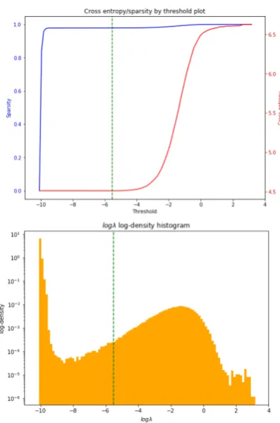
varia-Figure 1: Plots of validation cross-entropy (red line) of a LSTM model with a DSVI-ARD softmax layer on the PTB dataset and its corresponding sparsity (blue line) for different possible thresholdlogλthreshvalues (top) and the distribution histogram of its prior log-variances

logλij(bottom). We display the density on alog scale

due to a very sparse distribution. The threshold cho-sen for further model evaluation (the best in terms of perplexity on the validation set)logλopt_threshis marked with a green dashed line.

tional parameters µ,σ and all the other network parameters (including biases of the DSVI-ARD layers). Variational optimization is performed with the DSVI-ARD algorithm, which, in turn, only requires gradients of the log-likelihood and KL-divergence. Therefore, overall model training is a standard gradient optimization of parameters based on backpropagation (specifically, BPTT in the RNN case) with negative ELBO as the loss function.

train-Original model Dataset Architecture

Number of parameters, M

(Full / Softmax)

Removed parameters, %

(Full / Softmax) Perplexity Accuracy,_%

LSTM, (Zaremba et al.,2014)

PTB

Original 19.8 / 6.5 No compression 80.85 27.4% DSVI-ARD(ours) 13.4 / 0.14 32.1% / 97.8% 91.84 27.2% LR for Softmax, (Grachev et al.,2019) 14.5 / 1.19 26.8 % / 81.7 % 84.12 N/A TT for Softmax, (Grachev et al.,2019) 14.3 / 1.03 27.8 % / 84.2 % 88.55 N/A Wikitext2 Original 50.1 / 21.6 No compression 94.27 27.5%

DSVI-ARD(ours) 28.9 / 0.43 42.3% / 98.0% 103.54 27.6%

LSTM + tied weights, (Inan et al.,2016)

PTB Original 13.3 / 6.5 No compression 75.68 27.7% DSVI-ARD(ours) 7.4 / 0.66 44.0% / 89.9% 82.27 27.3% Wikitext2 Original 28.4 / 21.6 No compression 86.62 27.9% DSVI-ARD(ours) 8.7 / 1.94 69.3% / 91.0% 87.36 28.1%

LSTM, (Chirkova et al.,2018) PTB

Original 5.64 / 2.56 No compression 129.3 N/A VD, (Chirkova et al.,2018) 3.2 / 0.12 43.3 % / 95.5 % 109.2 N/A DSVI-ARD (Ours) 3.18 / 0.1 43.6 % / 96.1 % 106.2 25.9 %

Table 1: Language modeling experiments results. We provide the number of parameters left after pruning (in millions) and the achieved compression ratios (in percents) of the whole network and the softmax layer alone along with the final quality (perplexity and accuracy) on the test set for each evaluated model. The original (uncompressed) models quality is provided for comparison.

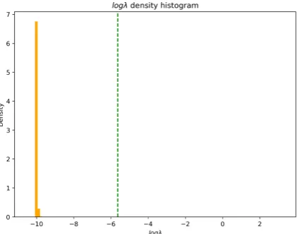
Figure 2: Distribution histogram of the prior log-variances logλij obtained for a LSTM model with a DSVI-ARD softmax layer on the PTB dataset. We pro-vide the standard-scaled density to justify the usage of a log scale in Fig.1(bottom).

ing procedure can be considered as pre-training on data (when the data term in ELBO dominates) and then starting fair optimization of the true ELBO (when the KL-weight reaches one). We used a simple linear KL-weight increasing strategy with a step selected as a hyperparameter.

During the evaluation of our models we do not sample parameters as we do in the training phase but instead set the approximated posterior mean

µ as DSVI-ARD layers weights. Then we zero

out the weights with the corresponding logarithms of prior variances lower than a certain threshold

logλthresh (a hyperparameter selected on

valida-tion):

logλ∗_ij <logλthresh ⇒µij := 0. (9)

This procedure essentially provides the desired sparsity as redundant weights are being literally removed from the network.

Each experiment was conducted as follows. We trained several models for some number of epochs with different hyperparameter initializa-tion (such as dropout rate, learning rate, etc.). Then we picked the best model in terms of cross-entropy (log-perplexity) on the validation set at the last training epoch. We did not zero weights during evaluation at this phase, in other words,

logλthresh =−∞in equation (9). After that, we

started threshold selection for the picked model: we iterated over possible values of logλthresh

from the “leave-all” to the “remove-all” extreme values and chose the one (denoted bylogλopt_thresh) at which the best validation perplexity was ob-tained. Finally, we evaluated the model on the test set using the chosen optimal thresholdlogλopt_thresh. In our results we report the achieved

compres-sion ratiocr=

PK i=1

PD j=11[logλ

∗

ij<logλ opt thresh]

KD ,

per-plexity and accuracy2on the test set.

5.2 Results

Table 1concludes all the results obtained during our experiments.

The comparison of DSVI-ARD with other dense layers compression approaches revealed

2_{By accuracy, we mean the fraction of correctly predicted}

that our models can exhibit comparable perplex-ity qualperplex-ity while achieving much higher compres-sion (inGrachev et al.(2019) case) and even sur-pass models based on similar Bayesian compres-sion techniques (inChirkova et al.(2018) case).

Also it can be seen that encoder-decoder weight tying helps to obtain higher overall compression (from almost45%to70%reduction of all model weights), due to a smaller number of parameters in the whole network, and even better results in both perplexity and accuracy on both datasets. Quality improvement after weight tying is a common case, however, we see that it helps to especially enhance the performance of our models (perplexity drops by almost 10 points in PTB case and more than

16points in Wikitext2 case), which gives grounds for the proposed combination of DSVI-ARD and weight tying.

One can argue that DSVI-ARD may lead to overpruning (Trippe and Turner,2018) because in all our experiments (except the last one, compar-ing with Chirkova et al. (2018) results) a slight quality drop in terms of perplexity can be ob-served. However, we specifically provide the test accuracy as well, in terms of which we achieve comparable or even better results than original models. We suggest that this effect might be caused by prediction uncertainty (or entropy) in-crease rather than model quality deterioration.

Fig. 1 demonstrates plots of cross-entropy (log-perplexity) and sparsity for different thresh-olds logλthresh — essentially the

compression-quality trade-off plot — and the log-scaled dis-tribution histogram of the decoder layer’s prior log-variances logλ∗_ij obtained for a DSVI-ARD

LSTM model trained on the PTB dataset. We

also provide the same distribution on the stan-dard scale (Fig. 2) for comparison. The dashed green line denotes the value of the chosen thresh-oldlogλopt_threshwhich provides the best validation perplexity. We can observe that the overwhelm-ing majority of weights in the last layer are indeed redundant, i.e., have small prior variances, do not contribute to the inference, and can be removed without harming much model performance. We argue that DSVI-ARD eliminates weights that ob-struct generalization while leaving only those ac-tually necessary for correct prediction.

6 Conclusion

In this paper we adopted the DSVI-ARD algo-rithm for compressing recurrent neural networks. Our main contributions are extending DSVI-ARD to the case of non-iid objects and combining it with the weight tying technique. In our ex-periments involving LSTM networks in language modeling tasks, we have managed to obtain sub-stantially high compression ratios at an acceptable quality loss. The proposed method turned out to be comparable to or even surpassing other com-pression techniques like matrix decomposition and variational dropout.

There are several possible avenues for future work. An intriguing application of the proposed DSVI-ARD method for RNNs is the compres-sion of current state-of-the-art models (Yang et al.,

2017;Dai et al., 2019), which require enormous amounts of memory and computational resources. At the same time, one of the drawbacks of the cur-rent Bayesian compression approaches is a lack of their expressive ability, i.e., most of them are based on oversimplified posterior approximations and prior distributions (e.g., factorized Gaussian), which may lead to overly rough estimates and overall model inefficiency. A rigorous study of this problem is required. Another possible direc-tion is bringing Bayesian framework into matrix decomposition-based methods as well. This fu-sion may lead to more effective and justified com-pression techniques.

Acknowledgments

The article was prepared within the framework of the HSE University Basic Research Program and funded by the Russian Academic Excellence Project ’5-100’.

References

Mart´ın Arjovsky, Amar Shah, and Yoshua Bengio. 2016. Unitary evolution recurrent neural networks. InProceedings of the 33nd International Conference on Machine Learning, ICML 2016, New York City, NY, USA, June 19-24, 2016, pages 1120–1128.

Yoshua Bengio, R´ejean Ducharme, Pascal Vincent, and Christian Janvin. 2003. A neural probabilistic lan-guage model. Journal of Machine Learning Re-search, 3:1137–1155.

Yoshua Bengio and Jean-S´ebastien Senecal. 2003.

In-ternational Workshop on Artificial Intelligence and Statistics, AISTATS 2003, Key West, Florida, USA, January 3-6, 2003.

Bradley P. Carlin and Thomas A. Louis. 1997.

BAYES AND EMPIRICAL BAYES METHODS FOR DATA ANALYSIS. Statistics and Computing, 7(2):153–154.

Wenlin Chen, David Grangier, and Michael Auli. 2016.

Strategies for training large vocabulary neural lan-guage models. InProceedings of the 54th Annual Meeting of the Association for Computational Lin-guistics, ACL 2016, August 7-12, 2016, Berlin, Ger-many, Volume 1: Long Papers.

Nadezhda Chirkova, Ekaterina Lobacheva, and Dmitry P. Vetrov. 2018. Bayesian compression for natural language processing. InProceedings of the 2018 Conference on Empirical Methods in Natural Language Processing, Brussels, Belgium, October 31 - November 4, 2018, pages 2910–2915.

Kyunghyun Cho, Bart van Merrienboer, Dzmitry Bah-danau, and Yoshua Bengio. 2014. On the properties of neural machine translation: Encoder-decoder ap-proaches. In Proceedings of SSST@EMNLP 2014, Eighth Workshop on Syntax, Semantics and Struc-ture in Statistical Translation, Doha, Qatar, 25 Oc-tober 2014, pages 103–111.

Zihang Dai, Zhilin Yang, Yiming Yang, Jaime G. Carbonell, Quoc V. Le, and Ruslan Salakhutdi-nov. 2019. Transformer-xl: Attentive language models beyond a fixed-length context. CoRR, abs/1901.02860.

Artem M. Grachev, Dmitry I. Ignatov, and Andrey V. Savchenko. 2019. Compression of recurrent neural networks for efficient language modeling. Applied Soft Computing, 79:354 – 362.

Song Han, Huizi Mao, and William J. Dally. 2015.

Deep compression: Compressing deep neural net-work with pruning, trained quantization and huff-man coding.CoRR, abs/1510.00149.

Sepp Hochreiter and J¨urgen Schmidhuber. 1997.

Long short-term memory. Neural Computation, 9(8):1735–1780.

Jiri Hron, Alexander G. de G. Matthews, and Zoubin Ghahramani. 2018. Variational bayesian dropout: pitfalls and fixes.CoRR, abs/1807.01969.

Hakan Inan, Khashayar Khosravi, and Richard Socher. 2016. Tying word vectors and word classifiers: A loss framework for language modeling. arXiv preprint arXiv:1611.01462.

Valery Kharitonov, Dmitry Molchanov, and Dmitry Vetrov. 2018. Variational dropout via empirical bayes. CoRR, abs/1811.00596.

Diederik P. Kingma, Tim Salimans, and Max Welling. 2015. Variational dropout and the local reparame-terization trick.CoRR, abs/1506.02557.

Christos Louizos, Karen Ullrich, and Max Welling. 2017. Bayesian compression for deep learning. InAdvances in Neural Information Processing Sys-tems, pages 3288–3298.

Zhiyun Lu, Vikas Sindhwani, and Tara N. Sainath. 2016. Learning compact recurrent neural networks. In 2016 IEEE International Conference on Acous-tics, Speech and Signal Processing, ICASSP 2016, Shanghai, China, March 20-25, 2016, pages 5960– 5964.

Stephen Merity, Caiming Xiong, James Bradbury, and Richard Socher. 2016. Pointer sentinel mixture models. CoRR, abs/1609.07843.

Tom´aˇs Mikolov. 2012. Statistical Language Models Based on Neural Networks. Ph.D. thesis, Brno Uni-versity of Technology.

Tomas Mikolov, Martin Karafi´at, Luk´as Burget, Jan Cernock´y, and Sanjeev Khudanpur. 2010. Recur-rent neural network based language model. In IN-TERSPEECH 2010, 11th Annual Conference of the International Speech Communication Association, Makuhari, Chiba, Japan, September 26-30, 2010, pages 1045–1048.

Dmitry Molchanov, Arsenii Ashukha, and Dmitry P. Vetrov. 2017. Variational dropout sparsifies deep neural networks. InProceedings of the 34th Inter-national Conference on Machine Learning, ICML 2017, Sydney, NSW, Australia, 6-11 August 2017, pages 2498–2507.

Sharan Narang, Erich Elsen, Gregory Diamos, and Shubho Sengupta. 2017. Exploring sparsity in recurrent neural networks. arXiv preprint arXiv:1704.05119.

Ofir Press and Lior Wolf. 2017. Using the output em-bedding to improve language models. In Proceed-ings of the 15th Conference of the European Chap-ter of the Association for Computational Linguistics, EACL 2017, Valencia, Spain, April 3-7, 2017, Vol-ume 2: Short Papers, pages 157–163.

Casper Kaae Sønderby, Tapani Raiko, Lars Maaløe, Søren Kaae Sønderby, and Ole Winther. 2016. How to train deep variational autoencoders and proba-bilistic ladder networks. CoRR, abs/1602.02282.

Michalis K. Titsias and Miguel L´azaro-Gredilla. 2014. Doubly stochastic variational bayes for non-conjugate inference. InProceedings of the 31th In-ternational Conference on Machine Learning, ICML 2014, Beijing, China, 21-26 June 2014, pages 1971– 1979.

Brian Trippe and Richard Turner. 2018. Overprun-ing in variational bayesian neural networks. arXiv preprint arXiv:1801.06230.

Zhilin Yang, Zihang Dai, Ruslan Salakhutdinov, and William W. Cohen. 2017. Breaking the softmax bot-tleneck: A high-rank RNN language model. CoRR, abs/1711.03953.

Wojciech Zaremba, Ilya Sutskever, and Oriol Vinyals. 2014. Recurrent neural network regularization.