Visualizing and Understanding Neural Machine Translation

Proceedings of the 55th Annual Meeting of the Association for Computational Linguistics, pages 1150–1159 Vancouver, Canada, July 30 - August 4, 2017. c2017 Association for Computational Linguistics Proceedings of the 55th Annual Meeting of the Association for Computational Linguistics, pages 1150–1159

Vancouver, Canada, July 30 - August 4, 2017. c2017 Association for Computational Linguistics

Visualizing and Understanding Neural Machine Translation

Yanzhuo Ding†_{Yang Liu}†‡∗_{Huanbo Luan}†_{Maosong Sun}†‡ †_{State Key Laboratory of Intelligent Technology and Systems}

Tsinghua National Laboratory for Information Science and Technology

Department of Computer Science and Technology, Tsinghua University, Beijing, China

‡_{Jiangsu Collaborative Innovation Center for Language Competence, Jiangsu, China}

[email protected], [email protected] [email protected], [email protected]

Abstract

While neural machine translation (NMT) has made remarkable progress in recent years, it is hard to interpret its inter-nal workings due to the continuous rep-resentations and non-linearity of neural networks. In this work, we propose to use layer-wise relevance propagation (LRP) to compute the contribution of each contextual word to arbitrary hid-den states in the attention-based encoder-decoder framework. We show that visu-alization with LRP helps to interpret the internal workings of NMT and analyze translation errors.

1 Introduction

End-to-end neural machine translation (NMT), which leverages neural networks to directly map between natural languages, has gained increasing popularity recently (Sutskever et al., 2014; Bah-danau et al., 2015). NMT proves to outperform conventional statistical machine translation (SMT) significantly across a variety of language pairs (Junczys-Dowmunt et al.,2016) and becomes the newde factomethod in practical MT systems (Wu et al.,2016).

However, there still remains a severe challenge: it is hard to interpret the internal workings of NMT. In SMT (Koehn et al.,2003;Chiang,2005), the translation process can be denoted as a deriva-tion that comprises a sequence of transladeriva-tion rules (e.g., phrase pairs and synchronous CFG rules). Defined on language structures with varying gran-ularities, these translation rules are interpretable from a linguistic perspective. In contrast, NMT takes an end-to-end approach: all internal infor-mation is represented as real-valued vectors or

∗_{Corresponding author.}

matrices. It is challenging to associate hidden states in neural networks with interpretable lan-guage structures. As a result, the lack of inter-pretability makes it very difficult to understand translation process and debug NMT systems.

Therefore, it is important to develop new meth-ods for visualizing and understanding NMT. Ex-isting work on visualizing and interpreting neu-ral models has been extensively investigated in computer vision (Krizhevsky et al.,2012; Mahen-dran and Vedaldi,2015;Szegedy et al.,2014; Si-monyan et al.,2014;Nguyen et al.,2015;Girshick et al., 2014; Bach et al., 2015). Although visu-alizing and interpreting neural models for natural language processing has started to attract attention recently (Karpathy et al., 2016; Li et al., 2016), to the best of our knowledge, there is no exist-ing work on visualizexist-ing NMT models. Note that the attention mechanism (Bahdanau et al.,2015) is restricted to demonstrate the connection between words in source and target languages and unable to offer more insights in interpreting how target words are generated (see Section4.5).

In this work, we propose to use layer-wise rel-evance propagation (LRP) (Bach et al., 2015) to visualize and interpret neural machine translation. Originally designed to compute the contributions of single pixels to predictions for image classi-fiers, LRP back-propagates relevance recursively from the output layer to the input layer. In con-trast to visualization methods relying on deriva-tives, a major advantage of LRP is that it does not require neural activations to be differentiable or smooth (Bach et al., 2015). We adapt LRP to the attention-based encoder-decoder framework (Bahdanau et al.,2015) to calculate relevance that measures the association degree between two ar-bitrary neurons in neural networks. Case studies on Chinese-English translation show that visual-ization helps to interpret the internal workings of

在 纽约 zai niuyue

</s>

in New York </s>

source words

source word embeddings

source forward hidden states

source backward hidden states

source hidden states

source contexts

target hidden states

target word embeddings

target words

attention

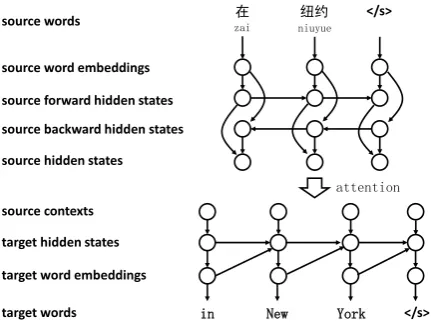
Figure 1: The attention-based encoder-decoder architecture for neural machine translation (Bah-danau et al.,2015).

NMT and analyze translation errors.

2 Background

Given a source sentence x = x1, . . . , xi, . . . , xI

with I source words and a target sentence y =

y1, . . . , yj, . . . , yJ with J target words,

neu-ral machine translation (NMT) decomposes the sentence-level translation probability as a product of word-level translation probabilities:

P(y_|x;θ) =

J

Y

j=1

P(yj|x,y<j;θ), (1)

wherey<j =y1, . . . , yj−1 is a partial translation. In this work, we focus on the attention-based encoder-decoder framework (Bahdanau et al., 2015). As shown in Figure1, given a source sen-tencex, the encoder first uses source word

embed-dings to map each source wordxito a real-valued

vectorxi.1

Then, a forward recurrent neural network (RNN) with GRU units (Cho et al.,2014) runs to calculate source forward hidden states:

− →_h

i=f(−→hi−1,xi), (2)

wheref(_·)is a non-linear function.

Similarly, the source backward hidden states can be obtained using a backward RNN:

←_h−

i=f(←−hi+1,xi). (3)

1_{Note that we usexto denote a source sentence andxto}

denote the vector representation of a single source word.

To capture global contexts, the forward and backward hidden states are concatenated as the hidden state for each source word:

hi= [−→hi;←−hi]. (4)

Bahdanau et al. (2015) propose an attention mechanism to dynamically determine the relevant source contextcj for each target word:

cj =

I+1

X

i=1

αj,ihi, (5)

where αj,i is an attention weight that indicates

how well the source wordxi and the target word

yj match. Note that an end-of-sentence token is

appended to the source sentence.

In the decoder, a target hidden state for thej-th target word is calculated as

sj =g(sj−1,yj,cj), (6)

whereg(_·) is a non-linear function,yj−1 denotes the vector representation of the(j₋1)-th target word.

Finally, the word-level translation probability is given by

P(yj|x,y<j;θ) =ρ(yj−1,sj,cj), (7)

whereρ(·)is a non-linear function.

Although NMT proves to deliver state-of-the-art translation performance with the capability to handle long-distance dependencies due to GRU and attention, it is hard to interpret the internal information such as −→hi, ←h−i, hi, cj, and sj in

the encoder-decoder framework. Though project-ing word embeddproject-ing space into two dimensions (Faruqui and Dyer,2014) and the attention matrix (Bahdanau et al.,2015) shed partial light on how NMT works, how to interpret the entire network still remains a challenge.

Therefore, it is important to develop new meth-ods for understanding the translation process and analyzing translation errors for NMT.

3 Approach

3.1 Problem Statement

in New York </s>

在 纽约 </s> in New

zai niuyue

Figure 2: Visualizing the relevance between the vector representation of a target word “New York” and those of all source words and preceding target words.

Girshick et al.,2014;Bach et al.,2015;Li et al., 2016). For example, in image classification, it is important to understand the contribution of a sin-gle pixel to the prediction of classifier (Bach et al., 2015).

In this work, we are interested in calculating the contribution of source and target words to the fol-lowing internal information in the attention-based encoder-decoder framework:

1. −→hi: thei-th source forward hidden state,

2. ←−hi: thei-th source backward hidden state,

3. hi: thei-th source hidden state,

4. cj: thej-th source context vector,

5. sj: thej-th target hidden state,

6. yj: thej-th target word embedding.

For example, as shown in Figure2, the gener-ation of the third target word “York” depends on both the source context (i.e., the source sentence “zai niuyue </s>”) and the target context (i.e., the partial translation “in New”). Intuitively, the source word “niuyue” and the target word “New” are more relevant to “York” and should receive higher relevance than other words. The problem is how to quantify and visualize the relevance be-tween hidden states and contextual word vectors.

More formally, we introduce a number of defi-nitions to facilitate the presentation.

Definition 1 Thecontextual word setof a hidden

state v ∈ RM×1 _{is denoted asC(v), which is a} set of source and target contextual word vectors

u_∈RN×1_{that influences the generation ofv.}

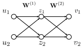
Figure 3: A simple feed-forward network for il-lustrating layer-wise relevance propagation (Bach et al.,2015).

For example, the context word set for −→hi

is {x1, . . . ,xi}, for ←h−i is {xi, . . . ,xI+1}, and for hi is {x1, . . . ,xI+1}. The contextual word set for cj is {x1, . . . ,xI+1}, for sj and yj is

{x1, . . . ,xI+1,y1, . . . ,yj−1}.

As both hidden states and contextual words are represented as real-valued vectors, we need to fac-torize vector-level relevance at the neuron level.

Definition 2 The neuron-level relevance

be-tween them-th neuron in a hidden statevm ∈ R

and the n-th neuron in a contextual word vector

un ∈ Ris denoted as run←vm ∈ R, which

satis-fies the following constraint:

vm=

X

u∈C(v)

N

X

n=1

run←vm (8)

Definition 3 Thevector-level relevance between

a hidden statev and one contextual word vector u_{∈ C}(v)is denoted asRu←v∈R, which quanti-fies the contribution ofuto the generation ofv. It is calculated as

Ru←v =

M

X

m=1

N

X

n=1

run←vm (9)

Definition 4 The relevance vector of a hidden

statev is a sequence of vector-level relevance of

its contextual words:

Rv={Ru1←v, . . . , Ru_|C(v)|←v} (10)

Therefore, our goal is to compute relevance vec-tors for hidden states in a neural network, as shown in Figure2. The key problem is how to compute neuron-level relevance.

3.2 Layer-wise Relevance Propagation

Input: A neural networkGfor a sentence pair and a set of hidden states to be visualizedV.

Output: Vector-level relevance setR. 1 foru∈Gin a forward topological orderdo 2 forv ∈OUT(u)do

3 calculating weight ratioswu→v;

4 end 5 end

6 forv∈ V do 7 forv ∈vdo

8 rv←v =v;// initializing neuron-level relevance

9 end

10 foru∈Gin a backward topological orderdo

11 ru←v =Pz∈OUT(u)wu→zrz←v;// calculating neuron-level relevance

12 end

13 foru_{∈ C}(v)do

14 Ru←v =Pu∈u

P

v∈vru←v;// calculating vector-level relevance

15 _R=_{R ∪ {}Ru←v};// Update vector-level relevance set

16 end 17 end

Algorithm 1:Layer-wise relevance propagation for neural machine translation.

LRP first propagates the relevance from the out-put layer to the intermediate layer:

rz1←v1 =

W(2)_1,1z1

W(2)_1,1z1+W2(2),1z2

v1 (11)

rz2←v1 =

W(2)_2,1z2

W(2)_1,1z1+W2(2),1z2

v1 (12)

Note that we ignore the non-linear activation func-tion because Bach et al. (2015) indicate that LRP isinvariantagainst the choice of non-linear func-tion.

Then, the relevance is further propagated to the input layer:

ru1←v1 =

W(1)_1,1u1

W(1)_1,1u1+W(1)2,1u2

rz1←v1 +

W(1)_1,2u1

W(1)_1,2u1+W(1)2,2u2

rz2←v1 (13)

ru2←v1 =

W(1)_2,1u2

W(1)_1,1u1+W(1)2,1u2

rz1←v1 +

W(1)_2,2u2

W(1)_1,2u1+W(1)_2,2u2

rz2←v1 (14)

Note thatru1←v1 +ru2←v1 =v1.

More formally, we introduce the following def-initions to ease exposition.

Definition 5 Given a neuronu, itsincoming

neu-ron set IN(u) comprises all its direct connected

preceding neurons in the network.

For example, in Figure3, the incoming neuron set ofz1isIN(z1) ={u1, u2}.

Definition 6 Given a neuron u, its outcoming

neuron setOUT(u)comprises all its direct

con-nected descendant neurons in the network. For example, in Figure3, the incoming neuron set ofz1isOUT(z1) ={v1, v2}.

Definition 7 Given a neuron v and its incoming

neurons u _∈ IN(v), the weight ratio that

mea-sures the contribution ofutovis calculated as

wu→v =

Wu,vu

P

u0_∈IN(v)Wu0,vu0 (15)

Although the NMT model usually involves multiple operators such as matrix multiplication, element-wise multiplication, and maximization, they only influence the way to calculate weight ra-tios in Eq. (15).

For matrix multiplication such asv = Wu, its

basic form that is calculated at the neuron level is given byv=P_u∈IN(v)Wu,vu. We follow Bach

近 两

jin liang

年 nian

来 lai

， 美国

, meiguo

近 两 年 来 ， 美国

jin liang nian lai , meiguo

1 2 3 4 5 6

1 2 3 4 5 6

Figure 4: Visualizing source hidden states for a source content word “nian” (years).

For element-wise multiplication such as v = u1◦u2, its basic form is given byv=Qu∈IN(v)u. We use the following method to calculate its weight ratio:

wu→v = P u

u0_∈IN(v)u0

(16)

For maximization such as v = max_{u1, u2}, we calculate its weight ratio as follows:

wu→v=

1 ifu= maxu0_∈IN(v){u0}

0 otherwise (17)

Therefore, the general local redistribution rule for LRP is given by

ru←v =

X

z∈OUT(u)

wu→zrz←v (18)

Algorithm 1 gives the layer-wise relevance propagation algorithm for neural machine trans-lation. The input is an attention-based encoder-decoder neural network for a sentence pair after decodingGand a set of hidden states to be visu-alized V. The output is a set of vector-level rel-evance between intended hidden states and their contextual words R. The algorithm first com-putes weight ratios for each neuron in a forward pass (lines 1-4). Then, for each hidden state to be visualized (line 6), the algorithm initializes the neuron-level relevance for itself (lines 7-9). After initialization, the neuron-level relevance is back-propagated through the network (lines 10-12). Fi-nally, vector-level relevance is calculated based on neuron-level relevance (lines 13-16). The time complexity of Algorithm1isO(_|G_|×|V|×Omax),

我 参拜 是 为了 祈求 my

wo canbai shi weile qiqiu

my₁ visit₂ is₃ to₄ pray₅

1 2 3 4 5 1

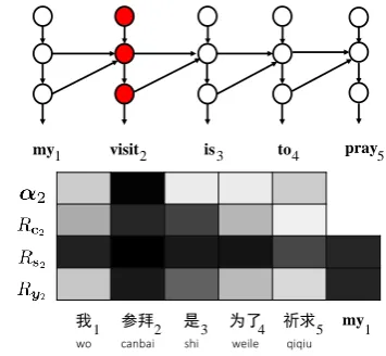
Figure 5: Visualizing target hidden states for a tar-get content word “visit”.

where|G_|is the number of neuron units in the neu-ral networkG,|V| is the number of hidden states to be visualized andOmaxis the maximum of out-degree for neurons in the network. Calculating relevance is more computationally expensive than computing attention as it involves all neurons in the network. Fortunately, it is possible to take ad-vantage of parallel architectures of GPUs and rel-evance caching for speed-up.

4 Analysis

4.1 Data Preparation

We evaluate our approach on Chinese-English translation. The training set consists of 1.25M pairs of sentences with 27.93M Chinese words and 34.51M English words. We use the NIST 2003 dataset as the development set for model selection and the NIST 2004 dataset as test set. The BLEU score on NIST 2003 is 32.73.

We use the open-source toolkit GROUNDHOG

(Bahdanau et al., 2015), which implements the attention-based encoder-decoder framework. Af-ter model training and selection on the training and development sets, we use the resulting NMT model to translate the test set. Therefore, the vi-sualization examples in the following subsections are taken from the test set.

4.2 Visualization of Hidden States 4.2.1 Source Side

the 𝐥𝐚𝐫𝐠𝐞𝐬𝐭 UNK in 𝐭𝐡𝐞 𝐰𝐨𝐫𝐥𝐝

zhaiwuguo 世界

2 3 4 5 6 7

最 大 的 债务国* ， the largest

2 3 4 5 6 7 2 3

de da zui

shijie ,

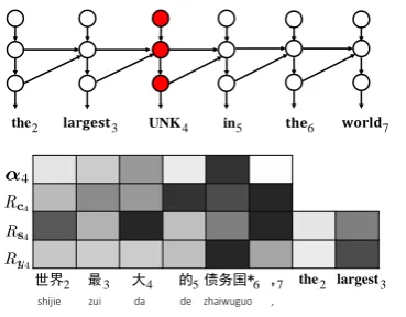
Figure 6: Visualizing target hidden states for a tar-get UNK word.

to denote the position of the word in the sentence. For example, “nian” (years) is the third word.

We are interested in visualizing the relevance between the third source forward hidden state−→h3 and all its contextual words “jin” (recent) and “liang” (two). We observe that the direct preced-ing word “liang” (two) contributes more to form-ing the forward hidden state of “nian” (years). For the third source backward hidden state ←h−3, the relevance of contextual words generally decreases with the increase of the distance to “nian” (years). Clearly, the concatenation of forward and back-ward hidden statesh3capture contexts in both di-rections.

The situations for function words and punctua-tion marks are similar but the relevance is usually more concentrated on the word itself. We omit the visualization due to space limit.

4.2.2 Target Side

Figure5visualizes the target-side hidden states for the second target word “visit”. For comparison, we also give the attention weightsα2, which cor-rectly identifies the second source word “canbai” (“visit”) is most relevant to “visit”.

The relevance vector of the source contextc2is generally consistent with the attention but reveals that the third word “shi” (is) also contributes to the generation of “visit”.

For the target hidden state s2, the contextual word set includes the first target word “my”. We find that most contextual words receive high val-ues of relevance. This phenomenon has been fre-quently observed for most target words in other sentences. Note that relevance vector is not nor-malized. This is an essential difference between

vote of confidence

参

6 7 8

众 两 院

5 6 7 8 9

yuan liang zhong can

in₉ the₁₀

senate the 10

senate₁₁ </s>₁₂

信任 投票 </s>_{11 10 11}

xinren toupiao </s>

Figure 7: Analyzing translation error: word omis-sion. The 6-th source word “zhong” is untrans-lated incorrectly.

attention and relevance. While attention is defined to be normalized, the only constraint on relevance is that the sum of relevance of contextual words is identical to the value of intended hidden state neuron.

For the target word embeddingy2, the relevance is generally consistent with the attention by iden-tifying that the second source word contributes more to the generation of “visit”. ButRy2 further indicates that the target word “my” is also very im-portant for generating “visit”.

Figure 6 shows the hidden states of a target UNK word, which is very common to see in NMT because of limited vocabulary. It is interesting to investigate whether the attention mechanism could put a UNK in the right place in the translation. In this example, the 6-th source word “zhaiwuguo” is a UNK. We find that the model successfully pre-dicts the correct position of UNK by exploiting surrounding source and target contexts. But the ordering of UNK usually becomes worse if multi-ple UNK words exist on the source side.

4.3 Translation Error Analysis

Given the visualization of hidden states, it is possi-ble to offer useful information for analyzing trans-lation errors commonly observed in NMT such as word omission, word repetition, unrelated words and negation reversion.

4.3.1 Word Omission

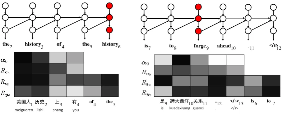
pro-the history of

美国人

2 3 4

历史 上 有

1 2 3 4 4

you shang lishi meiguoren

the₅ history₆

of the 5

Figure 8: Analyzing translation error: word repe-tition. The target word “history” occurs twice in the translation incorrectly.

duces a wrong translation “pakistani president win over democratic vote of confidence in the senate”. One translation error is that the 6-th source word “zhong” (house) is incorrectly omitted for transla-tion.

As the end-of-sentence token “</s>” occurs early than expected, we choose to visualize its cor-responding target hidden states. Although the at-tention correctly identifies the 6-th source word “zhong” (house) to be important for generating the next target word, the relevance of source con-textRc12 attaches more importance to the end-of-sentence token.

Finally, the relevance of target word Ry12 re-veals that the end-of-sentence token and the 11-th target word “senate” become dominant in the soft-max layer for generating the target word.

This example demonstrates that only using at-tention matrices does not suffice to analyze the internal workings of NMT. The values of rele-vance of contextual words might vary significantly across different layers.

4.3.2 Word Repetition

Given a source sentence “meiguoren lishi shang you jiang chengxi de chuantong , you fancuo ren-cuo de chuantong” (in history , the people of amer-ica have the tradition of honesty and would not hesitate to admit their mistakes), the NMT model produces a wrong translation “in the history of the history of the history of the americans , there is a tradition of faith in the history of mistakes”. The

is to forge ahead . </s>

</s> 是

7 8 9 10 11 12

跨大西洋 关系 。 </s> is to

9 10 11 12 13 6 7

. guanxi kuadaxiyang is

Figure 9: Analyzing translation error: unrelated words. The 9-th target word “forge” is totally un-related to the source sentence.

translation error is that “history” repeats four times in the translation.

Figure 8 visualizes the target hidden states of the 6-th target word “history”. According to the relevance of the target word embedding Ry6, the first source word “meiguoren” (american), the second source word “lishi” (history) and the 5-th target word “the” are most relevant to the gen-eration of “history”. Therefore, word repetition not only results from wrong attention but also is significantly influenced by target side context. This finding confirms the importance of control-ling source and target contexts to improve fluency and adequacy (Tu et al.,2017).

4.3.3 Unrelated Words

Given a source sentence “ci ci huiyi de yi ge zhongyao yiti shi kuadaxiyang guanxi” (one the the top agendas of the meeting is to discuss the cross-atlantic relations), the model prediction is “a key topic of the meeting is to forge ahead”. One translation error is that the 9-th English word “forge” is totally unrelated to the source sentence. Figure 9 visualizes the hidden states of the 9-th target word “forge”. We find that while the attention identifies the 10-th source word “kuadaxiyang” (cross-atlantic) to be most rele-vant, the relevance vector of the target wordRy9 finds that multiple source and target words should contribute to the generation of the next target word.

we will talk

就

11 12 13

谈 不 上

6 7 8 9 10

shang bu tan jiu

about₁₄development₁₅

talk will₁₂

发展 ₁₃

fazhan

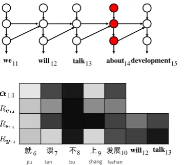
Figure 10: Analyzing translation error: negation. The 8-th negation source word “bu” (not) is not translated.

values in the relevance vector of the target word being generated.

4.3.4 Negation Reversion

Given a source sentence “bu jiejue shengcun wenti , jiu tan bu shang fa zhan , geng tan bu shang ke chixu fazhan” (without solution to the issue of sub-sistence , there will be no development to speak of , let alone sustainable development), the model pre-diction is “if we do not solve the problem of liv-ing , we will talk about development and still less can we talk about sustainable development”. The translation error is that the 8-th negation source word “bu” (not) is untranslated. The omission of negation is a severe translation error it reverses the meaning of the source sentence.

As shown in Figure10, while both attention and relevance correctly identify the 8-th negation word “bu” (not) to be most relevant, the model still gen-erates “about” instead of a negation target word. One possible reason is that target context words “will talk” take the lead in determining the next target word.

4.4 Extra Words

Given a source sentence “bajisitan zongtong mux-ialafu yingde can zhong liang yuan xinren tou-piao”(pakistani president musharraf wins votes of confidence in senate and house), the model predic-tion is “pakistani president win over democratic vote of confidence in the senate” The translation error is that the 5-th target word “democratic” is extra generated.

democratic vote of confidence

两

5 6 7 8

院 信任 投票 </s>

7 8 9 10 11

toupiao xinren yuan liang

in₉ the₁₀

win over

3 4

</s>

Figure 11: Analyzing translation error: extra word. The 5-th target word “democratic” is an ex-tra word.

Figure 11 visualizes the hidden states of the 9-th target word “forge”. We find that while the attention identifies the 9-th source word “xin-ren”(confidence) to be most relevant, the relevance vector of the target word Ry9 indicates that the end-of-sentence token and target words contribute more to the generation of “democratic”.

4.5 Summary of Findings

We summarize the findings of visualizing and an-alyzing the decoding process of NMT as follows:

1. Although attention is very useful for under-standing the connection between source and target words, only using attention is not suf-ficient for deep interpretation of target word generation (Figure9);

2. The relevance of contextual words might vary significantly across different layers of hidden states (Figure9);

3. Target-side context also plays a critical role in determining the next target word being gen-erated. It is important to control both source and target contexts to produce correct trans-lations (Figure10);

5 Related Work

Our work is closely related to previous visualiza-tion approaches that compute the contribuvisualiza-tion of a unit at the input layer to the final decision at the output layer (Simonyan et al., 2014; Mahen-dran and Vedaldi,2015;Nguyen et al.,2015; Gir-shick et al., 2014; Bach et al., 2015; Li et al., 2016). Among them, our approach bears most re-semblance to (Bach et al., 2015) since we adapt layer-wise relevance propagation to neural ma-chine translation. The major difference is that word vectors rather than single pixels are the ba-sic units in NMT. Therefore, we propose vector-level relevance based on neuron-vector-level relevance for NMT. Calculating weight ratios has also been carefully designed for the operators in NMT.

The proposed approach also differs from (Li et al., 2016) in that we use relevance rather than partial derivative to quantify the contributions of contextual words. A major advantage of using rel-evance is that it does not require neural activations to be differentiable or smooth (Bach et al.,2015).

The relevance vector we used is significantly different from the attention matrix (Bahdanau et al., 2015). While attention only demonstrates the association degree between source and target words, relevance can be used to calculate the as-sociation degree between two arbitrary neurons in neural networks. In addition, relevance is effective in analyzing the effect of source and target con-texts on generating target words.

6 Conclusion

In this work, we propose to use layer-wise rele-vance propagation to visualize and interpret neural machine translation. Our approach is capable of calculating the relevance between arbitrary hidden states and contextual words by back-propagating relevance along the network recursively. Analyses of the state-of-art attention-based encoder-decoder framework on Chinese-English translation show that our approach is able to offer more insights than the attention mechanism for interpreting neu-ral machine translation.

In the future, we plan to apply our approach to more NMT approaches (Sutskever et al.,2014; Shen et al.,2016;Tu et al.,2016;Wu et al.,2016) on more language pairs to further verify its effec-tiveness. It is also interesting to develop relevance-based neural translation models to explicitly con-trol relevance to produce better translations.

Acknowledgements

This work is supported by the National Natu-ral Science Foundation of China (No.61522204), the 863 Program (2015AA015407), and the National Natural Science Foundation of China (No.61432013). This research is also supported by the Singapore National Research Foundation un-der its International Research Centre@Singapore Funding Initiative and administered by the IDM Programme.

References

Sebastian Bach, Alexander Binder, Gr´egoire Mon-tavon, Frederick Klauschen, Klaus-Robert M¨uller, and Wojciech Samek. 2015. On pixel-wise explana-tions for non-linear classifier decisions by layer-wise relevance propagation. PLoS ONE.

Dzmitry Bahdanau, KyungHyun Cho, and Yoshua Bengio. 2015. Neural machine translation by jointly learning to align and translate. In Proceedings of ICLR.

Davie Chiang. 2005. A hierarchical phrase-based model for statistical machine translation. In Pro-ceedings of ACL.

Kyunghyun Cho, Bart van Merrienboer, Caglar Gul-cehre, Dzmitry Bahdanau, Fethi Bougares, Holger Schwenk, and Yoshua Bengio. 2014. Learning phrase representations using rnn encoder–decoder for statistical machine translation. In Proceedings of EMNLP.

Mannal Faruqui and Chris Dyer. 2014. Improving vec-tor space word representations using multilingual correlation. InProceedings of EACL.

Ross Girshick, Jeff Donahue, Trevor Darrell, and Jiten-dra Malik. 2014. Rich feature hierarchies for accu-rate object detection and semantic segmentation. In Proceedings of CVPR.

Marcin Junczys-Dowmunt, Tomasz Dwojak, and Hieu Hoang. 2016. Is neural machine translation ready for deployment? a case study on 30 translation di-rections. arXiv:1610.01108v2.

Andrej Karpathy, Justin Johnson, and Fei-Fei Li. 2016. Visualing and understanding recurrent networks. In Proceedings of ICLR Workshop.

Philipp Koehn, Franz J. Och, and Daniel Marcu. 2003. Statistical phrase-based translation. InProceedings of NAACL.

Jiwei Li, Xinlei Chen, Eduard Hovy, and Dan Jurafsky. 2016. Visualizing and understanding neural models in nlp. InProceedings of NAACL.

Aravindh Mahendran and Andrea Vedaldi. 2015. Un-derstanding deep image representations by inverting them. InProceedings of CVPR.

Anh Nguyen, Jason Yosinski, and Jeff Clune. 2015. Deep neural networks are easily fooled: High con-fidence predictions for unrecignizable images. In Proceedings of CVPR.

Shiqi Shen, Yong Cheng, Zhongjun He, Wei He, Hua Wu, Maosong Sun, and Yang Liu. 2016. Minimum risk training for neural machine translation. In Pro-ceedings of ACL.

Karen Simonyan, Andrea Vedaldi, and Andrew Zisser-man. 2014. Deep inside convolutional networks: Vi-sualizing image classification models and saliency maps. InProceedings of ICLR Workshop.

Ilya Sutskever, Oriol Vinyals, and Quoc V. Le. 2014. Sequence to sequence learning with neural net-works. InProceedings of NIPS.

Christian Szegedy, Wojciech Zaremba, Ilya Sutskever, Joan Bruna, Dumitru Erhan, Ian Goodfellow, and Rob Fergus. 2014. Intriguing properties of neural networks. InProceedings of ICLR.

Zhaopeng Tu, Yang Liu, Lifeng Shang, Xiaohua Liu, and Hang Li. 2017. Context gates for neural ma-chine translation. Transactions of the ACL.

Zhaopeng Tu, Zhengdong Lu, Yang Liu, Xiaohua Liu, and Hang Li. 2016. Modeling coverage for neural machine translation. InProceedings of ACL. Yonghui Wu, Mike Schuster, Zhifeng Chen, Quoc V.