Munich Personal RePEc Archive
Trends, Cycles and Lost Decades:
Decomposition from a DSGE Model with
Endogenous Growth
Hasumi, Ryo and Iibsoshi, Hirokuni and Nakamura, Daisuke
Japan Center for Economic Research, Graduate School of Social
Sciences, Tokyo Metropolitan University, Consumer Affairs Agency,
Government of Japan
31 January 2018
Trends, Cycles and Lost Decades
Decomposition from a DSGE Model
with Endogenous Growth
∗Ryo Hasumi†, Hirokuni Iiboshi‡, Daisuke Nakamura§
January 31, 2018
Abstract
In this paper we incorporate endogenous productivity growth into a medium-scale new Keynesian dynamic stochastic general equilibrium (DSGE) model, to which a new shock regarding R&D activities is added. By matching the model parameters to the Japanese economy from 1980:Q2 to 2013:Q4 and decomposing the output into trend and cycle components, we find that the stagnation of the so-called lost decades was caused by a decline in economic growth as well as major recessions in the busi-ness cycle. The common trend estimated by our model is based on multiple time series data and is much more volatile than the trend extracted by either the Hodrick-Prescott or the band-pass filter.
Keywords: endogenous TFP growth, New Keynesian DSGE, trend shift, techno-logical change
1
Introduction
After the bubble economy had reached the point of collapse in January 1991, the Japanese
economy experienced a long period of stagnation, the so-called “lost decades.” During
this period, two other economic crises occurred, specifically the Asian currency crisis in 1997 and the collapse of Lehman Brothers in 2008. These repeated crises are likely to
have made the growth rate of the real GDP reverse from upwards to downwards. The
∗The authors appreciate comments from Hiroki Arato, Kozo Ueda, Munechika Katayama, Takayuki
Tsuruga, Ryo Jinnai, and participants of 2016 Autumn meeting of Japanese Economic Association held at Waseda university in Tokyo. The views expressed herein are of our own and do not represent those of the organizations the authors belongs to.
†Japan Center for Economic Research
sources and magnitudes of the stagnation during the lost decades are analyzed by many
economists and policy makers. However, the topic seems to be controversial, and we can obtain no consensus for this debate. For instance, Hayashi and Prescott (2002) points
out that the slowdown of total factor productivity (TFP) must be a key factor in the long stagnation. This is because the stagnation should be regarded not as a decline caused
by temporary shocks mainly triggered by the demand side but as permanent shocks of
production. If so, it is plausible that there was a huge decline on the supply side but no change on the demand side behind this severe situation. In addition, Kaihatsu and
Kurozumi (2014) estimates the extent to which the financial accelerator of the banking
sector influenced the decline of the lost decades, but financial friction contributed a tiny portion to it in Japan.
On the other hand, central banks and policy organizations in developed countries
have aggressively adopted the dynamic stochastic general equilibrium model based on the new Keynesian (NK) framework to analyze business cycles and the effects of
mon-etary and fiscal policies on macroeconomics, particularly since the millennium. Earlier
empirical studies focusing on Japan, such as those by Sugo and Ueda (2008), Kaihatsu and Kurozumi (2014) and Iiboshi, Matsumae, Namba and Nishiyama (2015), determine
that the price and wage rigidities and habit formation of consumption assumed in NK
models are important factors to grasp comovements among economic series represent-ing business cycles as well as the variation in TFP. However, these models are set up
to focus on short-term rather than long-term frequency. Comin and Gertler (2006) open
a crack in this drawback. They incorporate the endogenous growth model proposed by Romer (1990) into a real business cycle (RBC) model and decompose the output series
between business cycles and trends in terms of the macroeconomic framework. Thanks
to their contribution, we can concentrate simultaneously on both sides – the short-term and long-term co-movements – of various macroeconomic series. For example,
Guerron-Quintana and Jinnai (2015) and Guerron-Guerron-Quintana, Hirano and Jinnai (2016) analyze financial crises’ impact on the growth rate of the Great Recession for the US economy
using the framework of Comin and Gertler (2006).
In this paper we extend the RBC model by Comin and Gertler (2006) to the NK framework and empirically analyze the long stagnation in Japan by estimating the
ex-tended model. In this sense we follow Ikeda and Kurozumi (2014), who expand Comin
and Gertler’s (2006) model by embedding price and wage rigidities and financial fric-tion. We incorporate the persistence of habit consumption and index rules of prices and
wages into Ikeda and Kurozumi (2014)’s model. Using this model, we extract the trend
component from the real GDP and classify the factors contributing to the growth from the historical decomposition for Japan after 1981:Q2. Since the historical
economic crises is attributed, we reconsider the sources of the lost decades from the
viewpoint of macroeconomics.
The contributions of our paper are as follows. (1) We estimate a medium-scale NK
model, which adopts nominal rigidities of prices and wages and habit formation of con-sumption and focuses on short-term fluctuations, to which the R&D endogenous growth
framework by Comin and Gertler (2006) is added. Our model adopts both sides of
short-run and long-short-run fluctuations by combining business cycle and growth models. In addi-tion, we conduct model selection between our model and a standard NK model without
the endogenous growth framework. (2) By embedding a new shock regarding R&D
ac-tivities and using estimated parameters, we empirically classify the factors that are attributable to the long stagnation. Specifically, we calculate the historical and variance
decompositions of the common trend and business cycle components. (3) This paper is
the first empirical attempt to apply Comin and Gertler’s (2006) model to Japan.
Our empirical findings are follows. First, from the model selection in terms of the
marginal likelihood of Japan’s recent data set, a standard NK model without the
en-dogenous growth model is superior to our model. However, the assumption of nominal rigidities of prices and wages is likely to work very well even for a long period, for
exam-ple over three decades, since the Calvo price and wage parameters are high values and
this model dominates its counterpart without the rigidities. Second, the R&D activity and investment shocks account for the majority of the business cycle components of the
real GDP and investment. However, the R&D shock affects investment and
consump-tion in opposite direcconsump-tions, while the investment shock affects them in the same direc-tion. Third, our estimated common trend fluctuates with considerable volatility, similar
to the trend of investment extracted by the Hodrick-Prescott (HP) and band-pass (BP)
filters. In contrast, the trend components of output and consumption of both the HP and the BP filter have little volatility. Fourth, two deep declines in the growth rate during the
Asian financial crisis in 1998 and the Lehman Brothers’ failure in 2008:Q3 caused not only major recessions in the business cycles but also stagnation of the economic growth.
The rest of our paper is organized as follows. Section 2 describes the motivation
of this study. Our model and estimation method are explained in Sections 3 and 4, respectively. Section 5 deals with the estimation results. We conclude in Section 6. In the
Appendix we show that the equilibrium conditions consist of the first-order conditions
2
Motivation
Growth Decline in the “Lost Decades”
Hayashi and Prescott (2002) emphasize that the huge decline of economic growth at the
beginning of the 1990s resulted from a substantial reduction of total factor productivity (TFP). On the other hand, other empirical studies support the idea that the long
stagna-tion in this period occurred due to the reluctance of financial institustagna-tions to finance the
corporate sector. Besides, R&D must be an important factor in realizing and sustaining strong economic growth. This paper focuses on the effect of TFP on growth along the
line of Hayashi and Prescott (2002) and attempts to decompose the time series of the
TFP into several aspects based on DSGE and growth models. The decomposition might provide a clue for identifying the sources of the ”lost decades.”
Common Stochastic Trend and Endogenous Growth
There is a large literature considering the theoretical and empirical aspects of non-stationary univariate and multivariate time series, including the random-walk process
and co-integration. Many empirical studies report that most macroeconomic series, such
as GDP, consumption and investment, follow a non-stationary process. Furthermore, other empirical studies estimate the decomposition between the cycle component and
the trend component, since macroeconomic series are thought to consist of a stationary
process regarded as business cycles and a non-stationary process indicating a stochastic trend or economic growth.
King, Plosser, Stock and Watson (1991) examines the long-run relationship made by permanent productivity shocks, regarded as shocks to the common stochastic trend
of output, consumption and investment based on RBC theory, using a co-integration
test. Altig, Christiano, Eichenbaum and Linde (2011) expands their research to a DSGE model to express a model-based co-integration system by including an investment-specific
shock with a random-walk process. Most of the latest DSGE models, for instance those
by Adolfson, Las´een, Lind´e and Villani (2007) and Christiano, Trabandt and Walentin (2011), follow their unit root technology shock, inducing the common stochastic trend.
This study also adopts their theory of the growth rate and expands it by
incorporat-ing an endogenous growth model. Generally speakincorporat-ing, primary macroeconomic indexes, such as output, consumption and investment per capita and real wage, are considered to
include the common stochastic trend,logAt, which makes a long-run stable relationship
among them, that is,
log(Ct/Nt) = ˜ct+ log At,
log(It/Nt) = ˜it+ log At,
log Wt= ˜wt+ log At,
wherey˜t,˜ct,˜itandw˜tare idiosyncratic stationary time series around the steady state
in-dicating business cycle components. According to Altig et al. (2011), the common
stochas-tic trend, log(At), follows a non-stationary autonomous process with I(1) and the first
difference of the trend is a stationary process,
logµAt =ρlogµAt−1+zt, for −1< ρ <1
wherelogµAt islogµAt = logAt−logAt−1, andztis an exogenous technology shock. On
the other hand, the trend of our model follows an endogenous process:
log At= log At−1+
λx
1−αlogµ
V t ,
whereµVt is the growth rate of the goods variety given as
µVt = (1−δa) + ∆a,t.
The constant term on the right hand side of the equation above, 1−δa, represents the
deterministic growth rate, and stochastic growth is generated from the dynamics of an
endogenous variable,∆a,t, defined as the additional goods variety.
The New Keynesian model mainly focuses on the contemporaneous cross-sectional
relation of the business cycle components, whereas the endogenous growth model focuses on the trend component. Our study evaluates aspects using the above strategy.
Four Potential Sources of the “Lost Decades”
In the following sections, we estimate the cause of the decline in economic growth during the “lost decades” through the lens of a DSGE model with endogenous growth. As
de-scribed above, the shift in the technology growth rate,µAt , is determined by the growth
rate of the goods variety,µV
t , whereas the additional goods variety,∆a,t, implemented by
R&D activity, is affected by structural shocks from economic activity and market
clear-ing. Hence, by measuring the contribution of structural shocks to the additional goods
growth. The shocks considered in our study are classified into the following four aspects:
• The effect of TFP and physical investment
• The effect of R&D investment
• The effect of consumption
• The effect of monetary and fiscal policies
We exclude the financial sector from our model, since it can be assumed to have an
indirect effect on economic growth via the above four paths. Accordingly, our study just focuses on the four direct effects on economic growth.
3
Model
Our model adopts Comin and Gertler (2006)’s endogenous growth framework by R&D
investment. Ikeda and Kurozumi (2014) expands it by embedding price and wage rigidi-ties and financial friction, and we follow this strategy. The novelty of our model is an
R&D success probability shock embedded in the R&D sector, which represents the
ef-ficiency of a firm’s R&D activities. Furthermore, the model incorporates consumption habits and index rules of prices and wages to improve the fitness of the consumption,
price and wage to the data.
In the model the economy consists of three sectors, namely R&D, producers and households, with seven agents. The R&D sector contributes to economic growth by
de-veloping innovative technology, bringing new products manufactured by the productive
sector. In this framework innovation increases the variety of intermediate goods to hold symmetry of the two relations among different goods firms, that is, (1) retail goods vs.
wholesale goods and (2) final goods vs. intermediate goods, as described below.
3.1 R&D Sector
Innovator
The innovator is assumed to be a representative agent who creates new innovation,Id,t,
which is useful for increasing the quantity of intermediate goods, Xf,t(h). To achieve
this, he uses retail goods,Yt. Then he sells the right to his innovation to an adopter, who
converts the innovation into newly developed final goods via intermediate goods.
LetZtbe his total stock of innovation andδzthe obsolescence rate of the stock. Then
we obtain this dynamics as
where Φt is the R&D productive parameter that transforms additional innovation into
stock.Φtis given as
Φt≡χz
Zt−1
At−1
ρ Zt−1
Id,t
1−ρ
, (2)
with0< ρ≤1and whereχz>0is a scale parameter. Atrepresents the level of
technol-ogy, and the technology progress rate of our model,µA
t, can be written as the logarithm
of its ratio: log(At/At−1). Eq.(2) shows the congestion effect of the innovation stock in
which a largerAt−1 than the steady state reduces the value of Φt. Since the innovator
faces perfect competition, he optimizes his profit and gains zero profit, satisfying the
no-arbitrage condition, such as
1 = Φt(1−δz)EtΛt|t+1Jt+1, (3)
whereEtΛt|t+1is the stochastic discount factor (SDF) of households andJtis the value of
the innovation described in the following part. Eq. (3) indicates the equivalent exchange between the innovation and the retail goods, of which the price is unity. From Eq.(1) and
Eq.(3) we obtain the dynamics of the innovator as
Id,t= (1−δz){Zt−(1−δz)Zt−1}EtΛt|t+1Jt+1. (4)
Adopter
The adopter is categorized as a representative agent who converts the available
technol-ogy acquired from the innovator into a new product of intermediate goods. To buy the right to the innovation, he obtains loans from households, and he tries to manufacture
a new product using the retail goods,Yt. If he is successful, he sells it to intermediate
goods producers.
The value of a premature product, which has not yet been adopted, to the adopter is
obtained as
Jt= max Ia,t
−Ia,t+ (1−δa)
λtPtV + (1−λt)EtΛt|t+1Jt+1 , (5)
where Ia,t is the cost of investment for adoption and δa is the obsolescence rate of the
adopted technology.λtis the success probability of converting the innovation into a new
product. PtV denotes the value of the adopter successfully developing a new product,
which indicates the present value of profit of the adopter. The success probability is an
endogenous variable given as
λt≡λ0
Vt−1
At−1
Ia,t
ωa
where λ0 > 0, ωa > 0, Vt denotes the stock of adopted innovation, or the variety of
final goods, andzλ
t is an autoregressive (AR) process of a structural shock regarded as
an R&D success probability shock. This shock represents the efficiency of the adopter’s R&D activities.
Since there is a spillover effect of technology, we assume that it has a certain degree
of inertia1. Eq.(6) also shows the congestion effect of adoption slowing down the speed
of accumulation ofVt. The link between the level of technology and the stock of adopted
innovationVtcan be expressed as
At=V
λx
1−α
t , (7)
where λx is the markup rate of the price of final goods Xt, as described below. The
increment,∆a,t, of the adopted technologyVtis given as
∆a,t≡(1−δa)λt(Zt−1−Vt−1), (8)
where the term in brackets is the stock of innovation that the adopter owns but has not
yet adopted, and the first-order condition for investment, Ia,t, by maximizing Eq. (5)
subject to Eq.(6) and Eq.(8), is written as
Ia,t=ωa(1−δa) λtPtV −λtEtΛt|t+1Jt+1
. (9)
From Eq.(5) and Eq.(9) we obtain the value of unadopted innovation as
Jt= (1−δa)(1−ωa)λtPtV +{1−(1−ωa)λt}EtΛt|t+1Jt+1
, (10)
whereJtis also used as the optimization of the innovator as in Eq.(3).
3.2 Productive Sector
Firms are divided into four groups – (i) retailers, (ii) wholesalers, (iii) final goods firms
and (iv) intermediate goods firms – based on the categories of goods generated in the pro-duction process. The wholesaler and intermediate goods firms face a specialized market
under monopolistic competition, but only the former follow a Calvo-style price setting.
The rest of the firms produce under perfect competition.
Relation among the Four Types of Goods
Before describing the producing agents, we show the relation among the four types of
goods as follows.
1The R&D success probability shock in our paper corresponds to the “barriers to technology adoption”
a). The retail goodsYtare produced by bundling the wholesale goodsYt(w)indexed by
w∈[0,1], based on the CES production function, as
Yt=
Z 1
0
Yt(w) 1 1+λp dw
1+λp
, (11)
whereλp >0denotes the net markup rate of the wholesale goods.
b). The wholesale goods Yt(w) are produced from the final goods Xf,t(w) indexed by
f ∈[0, Vt−1]andw∈[0,1]with equal amounts as
Yt(w) =Xf,t. (12)
c). The final goods Xf,t are produced by bundling the intermediate goods Xf,t(h)
in-dexed byh∈[0,1], based on the CES production function, as
Xf,t=
Z 1
0
Xf,t(h) 1 1+λx dh
1+λx
, (13)
whereλx>0is the net markup rate of the intermediate goods.
Retailer
The retailer is a representative agent who produces retail goodsYt by bundling a set of
wholesale goodsYt(w)indexed byw∈[0,1]. Then the retail goods are sold to households,
intermediate goods firms, innovators and adopters. Under the constraint of the CES
production function (11), the retailer maximizes his profit, given as
max {Yt(w)}
PtYt−
Z 1
0
Pt(w)Yt(w)dw, (14)
where Pt and Pt(w) denote the prices of the retail goods and the wholesale goods,
re-spectively. The FOC of the retailer’s profit-maximizing problem indicates the demand function of the wholesale goods, given as
Yt(w) =
Pt(w)
Pt
−1+λp λp
Yt, (15)
Wholesaler
There is a continuum of wholesalers, indexed by w ∈ [0,1]. Each type of wholesaler
production function (12), the wholesalers minimize their costs, written as
min {Xf,t}
Z Vt−1
0
Pf,tx Pt
Xf,tdf −M Ct(w)Yt(w) (16)
wherePf,tx denotes the price of the final goods andM Ct(w)means the marginal cost of
producing wholesale goods, respectively. The FOC of the wholesaler’s cost-minimizing
problem suggests the marginal cost function of the wholesale goods, given as
M Ct(w) =
Pf,tx Pt
. (17)
M Ct(w)does not depend on the indexation variablew, so the marginal costM Ctis
com-mon to each wholesaler. Hereafter, we denoteM Ct(w)asM Ct.
The relation between the wholesale goods and the final goods has been shown in
Eq.(12). Under the constraint of the demand function, Eq. (15), they maximize their
profit, written as
max {Pt(w)}
Et
∞
X
j=0
(ξpβ)j
ΛC t+j
ΛCt (
Pt(w)
Pt+j j
Y
k=1
πγp
t+k−1π1−γp−M Ct+j
)
Yt+j(w), (18)
where a fractionξp∈[0,1]of the firms follow the index rule,Ptγp =P
γp
t−1π1−γp, since they
do not have the chance to optimize the price. The remaining firms,1−ξp, can optimize
their price setting based on the profit function. ΛCt is the marginal utility of households
in terms of consumption, since the profit is measured from retail goods, regarded as the numeraire.
By solving the above profit maximization problem, we obtain the FOCs, which are
referred to as the price version of the new Keynesian Phillips curve consisting of the following four equations:
πo t
πt
= (1 +λp)
Ktp
Ftp, (19)
Ktp=M CtYt+ξpEtΛt|t+1
πγp
t π1−γp
πt+1
−
1+λp λp
Ktp+1, (20)
Ftp=Yt+ξpEtΛt|t+1
πγp
t π1−γp
πt+1
−λp1
Ftp+1, (21)
1 =ξp
πγp
t−1π1−γp
πt
!−1 λp
+ (1−ξp)
whereKtp andFtp denote the auxiliary variables defined recursively as the above Eq.(20)
and Eq(21). πo
t is the target price deviation from the actual price πto = Pto/Pt, and the
target pricePtois the optimal value derived from the price setting if the wholesalers are
given the chance to change their price.
Final Goods Firms
There is a continuum of final goods firms, indexed byf ∈ [ 0, Vt−1]. They produce final
goodsXf,t by bundling a set of intermediate goods Xf,t(h) indexed byh ∈ [ 0,1 ],. Then
the final goods are sold to wholesale goods firms with nominal rigidity due to monopolis-tic competition. Under the constraint of the CES production function (13), a final goods
firm maximizes its profit, given as
max {Xf,t(h)}
Pf,tx Xf,t−
Z 1
0
Pf,tx (h)Xf,t(h) dh, (23)
where Px
f,t and Pf,tx (h) denote the prices of the final goods and the intermediate goods,
respectively. The FOC of the final goods firm indicates the demand function of the
inter-mediate goods, given as
Xf,t=
Pf,tx (h)
Px f,t
!−1+λx λx
Xf,t(h), (24)
In addition, we obtain the price equation of the final goods as
Pf,tx =
Z 1
0
Pf,tx (h)−λx1 dh −λx
. (25)
Intermediate Goods Firms
There is a continuum of intermediate goods firms, indexed byh ∈ [0,1], each of which
is produced using labor,lt(h), the physical capital stock service, ukt(h)Kt−1(h), and the
variety of all final goods, Vt, where ukt is the capital utilization rate. We assume that
the stock of adopted innovation Vt is also assumed to be the variety of the final goods
accumulated from new products.
We assume that each type of firm h adopts the Cobb-Douglas production function,
that is, uk
t(h)Kt−1(h)α(lt(h) )1−α=R0Vt−1 Xf,t(h) df, and that a new product,∆Vt,
ac-quired from the adopters increases the quantity ofXf,t(h)on the aggregated level, such
as ukt Kt−1
α
(lt)1−α =
R1
0
RVt−1
0 Xf,t(h) df dh, even though it uses the same levels of
in-puts,Kt(h)andl(h). By substituting Eq.(24) into it, we obtain the aggregated production
ukt(h)Kt−1(h)
α
(lt(h) )1−α =
Z Vt−1
0
Pf,tx (h)
Px f,t
!−1+λx λx
Xf,tdf. (26)
The depreciation rate of the capital also includes the adjustment cost, and it is writ-ten as
δukt≡δk+bk
ukt1+ζk
1 +ζk
, (27)
whereδk andbkrepresent the scale parameters of the capital depreciation function and
meet the equationsδk =δ− 1+bkζk and bk = µ
A
β +δ−1, respectively. The dynamic of the
capital accumulation is standard:
Kt=
1−δuktKt−1+ztiS(It/It−1)It (28)
wherezit is the measured productivity of investment, which is referred to as the AR (1)
process of the investment efficiency shock, andS(·)is an adjustment cost function with
respect to investment. In addition, the variety of intermediate goods accumulated by the adopted innovation has a dynamic such as
Vt = (1−δa)Vt−1+{1−Sa(∆a,t/∆a,t−1)}∆a,t, (29)
whereδais the obsolescence rate of the stock andSa(·)is a monotonically increasing
func-tion of the adjustment cost with respect to the difference of volume of the R&D variety
goods. The intermediate firm has to buy new adopted innovation∆a,t to compensate for
this obsolescence. Accordingly, by summing up all the activities of the firm, we express
its budget constraint as
Wt(h)lt(h) +rktukt(h)Kt−1(h) +PtV∆a,t(h) =
Z Vt−1(h)
0
Px f,t(h)
Pt
Xf,t(h) df, (30)
where the LHS and the RHS denote the cost and the revenue of the firms, respectively. The intermediate goods firms maximize the net present value of the profit by
con-trolling the price of intermediate goods, Pf,tx (h), the capital stock, Kt(h), the capital
utilization rate, uk
t(h), the labor demand, lt(h), the new product stock, Vt(h), and its
current dividendDt, so their optimization problem is obtained as
max {Px
h,t,Kt,ukt,lt,Vt,Dt}
Et
∞
X
j=0
βjΛ
C t+j
ΛC t
" RV t−1(h)
0
Px f,t(h)
Pt Xf,t(h) df−Wt(h)lt(h)
−rktukt(h)Kt−1(h)−PtV∆a,t(h)
#
subject to Eq.(26) through Eq.(30). The FOCs of the optimization problem consist of five
equations, as shown below.
Firstly, from the viewpoint of optimal pricing, the intermediate goods price meets
Pf,tx (h)
Pt
= (1 +λx)st. (32)
wherest is the Lagrangian multiplier in the production function Eq.(26), and it means
the shadow price of intermediate goods or the relative price of intermediate goods to retail goods, since the retail goods price is the numeraire in this paper.
Secondly, the FOC with respect to fixed capital rental cost,rkt, is given as
rtk=αst
uktKt−1
lt
α−1
, (33)
where the effective capital equipment ratio, uktKt−1
lt , is common to all intermediate firms,
so we omit the indexhfor simplicity.
Thirdly, the FOC of the labor demand,lt(h), is obtained as
Wt= (1−α)st
uk
tKt−1
lt
α
. (34)
Fourthly, the FOC with respect to newly adopted innovation,∆a,t, is written as
PV t =Γta
n
1−S′
a
∆ a,t(h)
µV∆ a,t−1(h)
−S′
a
∆ a,t(h)
µV∆ a,t−1(h)
∆ a,t(h)
µV∆ a,t−1(h)
o
+µVEtΛt|t+1Γta+1Sa′
∆a,t+1(h) µV∆
a,t(h)
∆a,t+1(h) µV∆
a,t(h)
2 , (35)
whereΓtais the Lagrangian multiplier of the firm’s accumulation of newly adopted
inno-vation. The FOC with respect to the stock of goods variety is obtained as
Γta=EtΛt|t+1
"
(1−δa)Γta+1+λxst+1
ukt+1Kt
α
(lt+1)1−α
Vt
#
, (36)
wherePtV is the value of the adopted innovation which is also used in the adopter’s value
function (5) described in the previous subsection.
We omit the price dispersion of wholesale goods, unlike Ikeda and Kurozumi (2014), since we have to use a log-linearized DSGE model to estimate it rather than a
non-linearized one. Hence, the quantity of aggregated final goods is equal to those of the
wholesale goods and retail goods, such asXf,t =Yt(w) =Yt. Finally, after substituting
Xf,t(w) =Ytand Eq.(7) into the Cobb-Douglas production function, uktKt−1
α
Xf,t, we obtain
Yt=
ukt Kt−1
α t V λx 1−α
t−1 lt
1−α, (37)
The appendix shows the derivation of the production function (37).
3.3 Households
There is a continuum of households, indexed byg∈[0,1]. However, when the households
face problems maximizing their intertemporal utility, they are regarded as a represen-tative agent that attains utility from consumption and leisure. Households’ preference
is given as
max {Ct,Bt,Kt,It}
E0βtztb
∞
X
t=0
(
ln (Ct−h Ct−1)−ztlγl
l1+ωl
t
1 +ωl
)
, (38)
whereCtandltdenote the aggregate consumption and labor supply, respectively. We also
allow for habit persistence in their preference by addingh Ct−1.ztb andzltare the
prefer-ence shock and labor supply shock, respectively. The budget constraint of households is given as
Ct+It+
Bt
Pt
+ Πt=rtkuktKt−1+Wtlt+rtn−1
Bt−1
Pt
+Tt, (39)
whereBt,TtandΠtare the bond holding and the lump sum public transfer and dividend
(or profit) of the productive sector, respectively. Wt is the real wage. Accordingly, by
solving the above problem, the first-order condition (FOC) in terms of consumption is
given as
ΛCt = z
b t
Ct−hCt−1
−βhEt
ztb+1 Ct+1−hCt
, (40)
where ΛC
t is the marginal utility with respect to consumption. In a similar way, the
FOCs in terms of bonds are obtained as
Λt|t+1 ≡βEtΛ
C t+1
ΛC t
, (41)
Λt|t+1 = Etπt+1
rn t
, (42)
where Λt|t+1 is the marginal utility with respect to bonds. Eq. (41) shows thatΛt|t+1
is the bond price measured by the shadow price of consumption goods, and it is also
Households are also fixed capital holders, and they optimize the capital holding,Kt,
investment, It, and capital utilization rate, ukt, to maximize the intertemporal utility.
The FOCs in terms of fixed capital and investment are given as
qkt =EtΛt|t+1
h
rkt+1ukt+1+qtk+1n1−δukt+1oi (43)
1 =zitqkt n1−S It
It−1
−S′ It
It−1
It
It−1
o
+EtΛt|t+1zti+1qkt+1S′
It+1 It
It+1 It
2 (44)
rtk=qtkδ′ukt (45)
whereqkt is the Tobin’s Q, which satisfiesqkt ≡ Λkt
ΛC t
.
Wage Setting
The households indexed by g ∈ [0,1] face monopolistic competition for supplying their
specialized labor, and their wage-setting problem possesses the property of nominal
rigidity, following Erceg, Henderson and Levin (2000). When households decide their
wage with the intermediate goods firms, they maximize the present value of the stream of their utilities as
max {Wg,t}
Et
∞
X
j=0
(βξw)j
(
ΛCt+jlg,t+j(µA)jWg,t j
Y
k=1
πγw
t+k−1π1−γw
πt+k
!
−γlztb+jztl+j
l1+ωl
g,t+j
1 +ωl
)
, (46)
where a fraction ofξw ∈[0,1]of households follow an index rule,PtγwWg,t=Ptγ−w1Wg,t−1π1−γw,
since they do not have the chance to optimize their wage. The remaining households,
1−ξw, conduct optimal wage setting. µAis the steady state of the technology progress
rate. The link between the specialized labor supply of each type of household and the aggregate labor supply is given by
lg,t=
Wg,t
Wt
−1+λw λw
lt, (47)
whereλw >0is the net markup rate of the real wage. By solving the above maximization
problem, we obtain the FOCs, which are referred to as the wage version of the new Keynesian Phillips curve consisting of the following four equations:
Wo t
Wt
=
(1 +λwztw)
Kw t
Ftw
λw
λw+ω+λw ω
Ktw =γlzbtztllt1+ω+Etβξw µA
πγw
t−1π1−γw
πt
Wt
Wt+1
!−1+λw λw (1+ω)
Ktw+1, (49)
Ftw=ΛCt Wtlt+Etβξw µA
πγw
t−1π1−γw
πt
Wt
Wt+1
!− 1 λw
Ftw+1, (50)
1 =ξw µA
πγw
t−1π1−γw
πt
Wt
Wt+1
!− 1 λw
+ (1−ξw)
Wo t Wt − 1 λw , (51)
whereWo
t is the target wage, which is the optimal solution derived from the wage-setting
problem when the households are given the chance to change their wage, and we add a
wage markup shock,zw
t , to the RHS of Eq.(48).
3.4 Other Equations
Market Clearing Condition
The aggregate output in the whole economy is composed of the sum of the demand for the retail goods. The market-clearing condition of the retail goods is given as
Yt=Ct+It+Ia,t(Zt−1−Vt−1) +Id,t+g/y ztg, (52)
where the third term is the investment of the adopters and the fourth term is the R&D
investment of the innovators.zgt denotes exogenous expenditure, such as the government
sector. However, each term in the equation does not necessarily match the data that we
use for estimation.
Since the real GDP with the benchmark year 2005 does not contain the R&D
in-vestment as its component, we use the following definition of output in the observation
equation explained in Section 4:
˜
Yt=Ct+It+g/y ztg. (53)
Monetary Policy
The central bank follows a Taylor-type monetary policy rule given as
lnrtn=φrlnrtn−1+ (1−φr)
lnrn+φπln
πt π
+φyln
yt
y
+εrt, (54)
where φr ∈ [0,1)denotes the degree of policy rate smoothing. φπ and φy are policy
re-sponses to inflation and output, respectively. εr
t is a monetary policy shock with an iid
Equilibrium Conditions and Structural Shocks
To acquire an equilibrium of the model and to estimate it, we use equations such as
Eq.(1) through Eq.(3), Eq.(6) through Eq.(10), Eq.(19) through Eq.(22), Eq.(26) through Eq.(30), Eq.(32) through Eq.(37), Eq.(40) through Eq.(42), and Eq.(48) through Eq.(54).
There are eight structural shocks, of which all shocks except the monetary policy shock
follow the AR (1) process. The appendix presents the conditions and the shocks.
3.5 Two Alternative Models
To investigate the properties of the decomposition obtained by our model, we introduce two alternative models. One is a “model without nominal rigidities” from which we
remove the assumptions of nominal rigidities in price and wage setting from the above
original model by setting the Calvo parameters of both nominal rigidities to zero. The other model is a standard New Keynesian model, which replaces the exogenous growth
rate, µzt, by removing the assumption of endogenous growth explained in Section 3.1
from the original model. The law of motion of the exogenous growth rate is defined as
log(µzt/µz) =ρzlog(µzt−1/µz) +εzt (55)
whereµz is the steady-state growth rate corresponding toµAin the endogenous growth
model andεz
t is a technology shock following an iid process. Hereafter, we refer to this
model as the “standard NK model.”
Thus, we compare the properties of the technology progress rate in the endogenous growth New Keynesian model (or “benchmark mode” in our paper) with that in the
stan-dard NK model to evaluate the performance of the endogenous growth mechanism as
the low-pass filter extracting the common trend component of economic fluctuations.
4
Estimation Strategy
This section describes the estimation strategy, including the data and the link between
the endogenous and the observable variables.
4.1 Estimation Methods
In this paper the values of the model parameters are estimated following a Bayesian approach via Markov chain Monte Carlo (MCMC) simulation. We use a stylized solution
method for estimation; specifically, we log-linearize the model shown above and convert
value of the likelihood obtained from the Kalman filter with a prior density. We generate
3 chains composed of 125,000 draws from the posterior distribution of the parameters by the Metropolis-Hastings algorithm and discard the first 20 percent of them (i.e. 20,000
draws) as burn-in iterations.
4.2 Observable Variables and Data
As can be seen from Table 1, we adopt seven observed variables – (1) output growth, (2) consumption, (3) investment, (4) retail goods price, (5) real wage, (6) labor supply and
(7) nominal interest rate, for Japan from 1980:Q2 through 2013:Q4. We collect the real
GDP,Ytdata, real private consumption,Ctdata, and fixed capital formation,Itdata, from the
Cabinet Office’s National Accounts as output, consumption and investment. We use the
2005 benchmark data that cover the period 1980:Q1–2013:Q4.
To make these demand series per capita, we divide them by the labor force, Nobs
t . As the price level, we use the implicit GDP deflator index from the Cabinet Office. The
worked hour indices,lobst , and the real wage indices, Wtobs, of the Monthly Labor Survey
are used for the labor supply,lt, and real wage,Wt. As the nominal interest rate, we use
the Bank of Japan’s secured overnight call rate.
[ Insert Table 1 ]
4.3 Link between Observable and Endogenous Variables
The equilibrium conditions of the model are rewritten in terms of detrended variables
around the steady state, and the detrended variables are given asyt = AYt−t1,Y˜t =
˜
Yt
At−1,
ct= ACt−t1,it= It
At−1,w o t = W
o t
At−1,wt= Wt
At−1,kt= Kt
At−1,mct= M Ct
(At−1)1−α
,st= (A St
t−1)1−α
,pVt =
PV t Vt−1
At−1 ,id,t = Id,t
At−1,λ c
t = ΛCt At−1,γa,t = Γa,tAVt−t−11,∆˜a,t = V∆t−a,t1,at−1 = ZVt−t−11,ia,t = Ia,tAt−Vt−11,
jt = JAtVt−t−11, φt = ΦVtAt−t−11, kpt = AKt−t1, f p
t = AFt−t1, k w
t = AKt−t1, f w
t = AFt−t1, µ A
t = AAt−t1, and
µVt = Vt
Vt−1.
The links between the observable and the endogenous variables are given as follows:
1. Real GDP Growth Rate
∆Ytobs = Y
data t /Ntdata
Ydata t−1 /Nt−data1
=µAt−1 × Y˜t ˜ Yt−1
. (56)
2. Real Private Consumption Growth Rate
∆Ctobs = C
data t /Ntdata
Cdata t−1/Nt−data1
=µAt−1 × ct
ct−1
3. Real Private Investment Growth Rate
∆Itobs = I
data t /Ntdata
Idata t−1/Nt−data1
=µAt−1 × it
it−1
. (58)
4. Real Wage Growth Rate
∆Wtobs= W
data t
Wdata t−1
=µAt−1 × wt
wt−1
. (59)
5. Labor Supply
ltobs= l
data t
100 = ¯l ×lt. (60)
6. Nominal Interest Rate
rn,obst = 1 +R
n,data t
400 =r
n
t. (61)
7. Price Inflation Rate
πtobs ≡ P
data t
Pdata t−1
=πt. (62)
The first four observable variables are the first difference of the data. µAt is the
loga-rithm of the common growth rate, that is,log (At/At−1). The annualized nominal rate is
changed to a quarterly basis by dividing it by 400. Notice that the first four equations indicate that those variables have a long, stable relation with the stochastic common
trend,At, as described in Section 2.2.
4.4 Calibrated Parameters and Prior Distribution
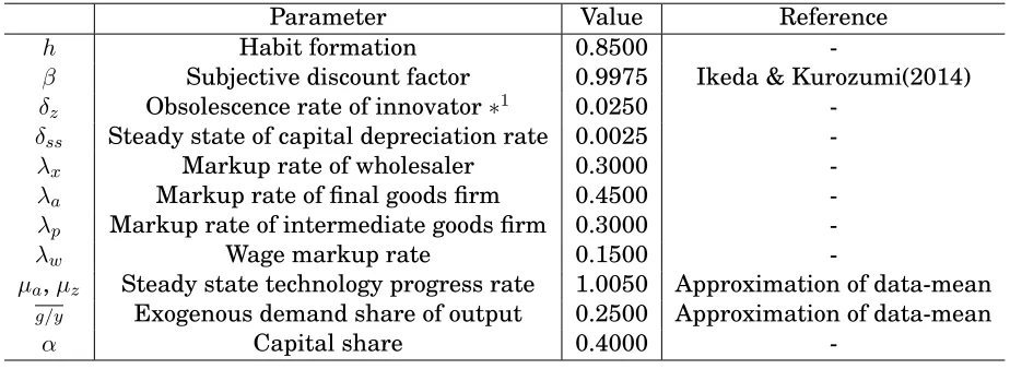
In this model we fix 11 parameters in Table 2 to avoid identification problems. The
steady state of the exogenous demand share of the output, including government,g/y, is
set to 0.25. The depreciation rates of the physical capital stock,δ, and the capital share,
α, are set to 0.025 and 0.4, respectively. The subjective discount rate, β, is closer to 1
than in recent studies of the Japanese economy, since the monetary policy rate has been permanently rather than temporarily close to 0 since 1999:Q1.
The prior distribution of the parameters to be estimated is described in the third through the fifth column of Table 3.
[ Insert Table 2 ]
5
Empirical Results and Discussion
5.1 Estimated Parameters
The estimations of the parameters of the benchmark model as well as the two alternative models are summarized in Table 3. To focus on growth as well as business cycles, we
expand the sample period to over thirty years, although it includes the period of the zero
interest rate policy (ZIRP). According to Hirose and Inoue (2016), the estimation bias of the ZIRP is not large and is acceptable when adopting a Taylor-type linear monetary
policy rule. To test the convergence of the MCMC sampling, we conduct Gelman and
Rubin (1992)’s convergence diagnostic and confirm the convergence of all the parameters, and we compare the empirical results of our benchmark model with those of the standard
NK model, the growth part of which is mainly based on that of Altig et al. (2011).
There are three remarks to make. First, we observe very similar values in the com-mon parameters of the three models except for the following results. The coefficient of
the investment adjustment cost is around 3.4 in the benchmark model, while it is 6.0
in the no nominal rigidity model and 8.3 in the NK model. This is because the common
trend,µAt−1, of the benchmark model moves more smoothly than that of the NK model.
Larger adjustment costs are more likely to work to offset fluctuations in the common
trend growth. In the no nominal rigidity model, it is observed that the inverse of the elasticity of the labor supply is 37.2 and the parameter of monetary policy smoothing is
0.1, since the classical dichotomy is held in the no nominal rigidity model, in which both
the Calvo price and the Calvo wage parameter are set to zero. The assumption causes the monetary policy to be ineffective, as indicated by the variance decomposition of the
business cycles in Table 6.
Second, the standard deviation of the success probability shock in the two
endoge-nous growth models is similar to that of the TFP shock in the NK model, although the
persistence of the former shock is a high value, such as 0.92 to 0.97, whereas that of the latter shock is 0.28. These differences affect the difference in the variance decomposition
of the business cycles between the three models, as described later in Table 6.
Third, we compare the estimation of our three models with previous Japanese stud-ies, such as those by Sugo and Ueda (2008) and Kaihatsu and Kurozumi (2014), who limit
the sample period to before the ZIRP. The Calvo price parameter of this study is nearly
0.96, and the Calvo wage parameter is around 0.65, whereas Sugo and Ueda (2008) esti-mate them to be 0.88 and 0.52 and Kaihatsu and Kurozumi (2014) estiesti-mate them to be
0.68 and 0.50, respectively. Through 3 studies focusing on Japan, we see that the Calvo
result is 0.96, while in Sugo and Ueda (2008) it is 0.10 and in Kaihatsu and Kurozumi
(2014) it is 0.26. This discrepancy might come from differences in the procedure followed for detrending the data and the sample period. Sugo and Ueda (2008) uses the HP filter
for detrending, whereas we do not use such a filter. The fluctuations in inflation are observed to be much smaller during the period of the ZIRP than during other periods,
which make habit formation more persistent under a constant price level.
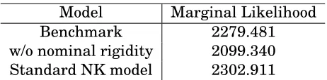
Table 4 shows the marginal likelihoods of the three models. When we use even prior model odds for the three models, the posterior odds of the benchmark model to the no
nominal rigidity model are one, which suggests that the nominal rigidities of price and
wage are significant. However, when we expand the model selection to a choice between three models, the NK model overwhelmingly dominates the other models with an
en-dogenous growth framework. The smoothness of each trend estimated by the models
with endogenous growth, which can be seen in panel (a) of Figure 2, might worsen the data fitting.
[ Insert Table 3 and Table 4 ]
5.2 Impulse Response
Before comparing the business cycle and common trend components of each model, we check the impulse response of the endogenous variables to a success rate shock. Figure
1 shows the impulse responses of endogenous variables to a one standard deviation
suc-cess rate shock: the solid lines are those of the benchmark model and the dash-dotted lines are those of the model without nominal rigidity. All the parameters are set to the
posterior mean described in Table 3.
[ Insert Fig. 1 ]
Panel (a) shows the impulse responses of the detrended variables,yˆt,cˆt,ˆit,ˆlt,ˆiRDt and
ˆ
µt, where R&D investment,iRDt , is defined as
iRDt =iat
1
at−1
−1
+idt (63)
A success rate shock increases the goods variety, Vt, as can be seen from Eq.(8), and
hence the level of technology rises. This effect is reflected in the increase in the
tech-nology progress rate,µt. Besides this direct effect, a success rate shock stimulates R&D
investment, as an increase in adoption due to the improvement of the success
proba-bility,λt, decreases the stock of the idea Zt and increases the value of innovation. The
not react with the model without nominal rigidity depends on the estimated
parame-ters rather than the characteristics of the model. The labor supply in the benchmark model changes to the positive direction in the short run in response to the increase in
productivity, as in the conventional wage rigidity model.
In Panel (a) it seems thatyˆt,ˆctandˆitmove irrelevantly and there is no co-movement
at first glance, but notice that these are detrended variables. Panel (b) shows the
devia-tion ofYˆt,Cˆt,IˆtandIˆtRD from the balanced growth path (trend of growth) when a success
rate shock has occurred. The cumulative amount ofµA
t is added to each series of Panel
(a). From the perspective of the deviation from the balanced growth path, the increase
in the rate of technological progress caused by a success rate shock increases the output, as is usually considered. It is also confirmed that consumption and investment co-move
with the output, suggesting that the success rate shock of our model plays a role similar
to the TFP shock of a conventional model. However, in addition to the direct effect of increasing the goods variety, there is an indirect effect of stimulating R&D investment.
5.3 Business Cycle and Common Trend Components
We evaluate the business cycle components and trend components of output,
consump-tion and investment derived from our estimaconsump-tion of the three DSGE models by
compar-ing them with those of the Hodrick-Prescott (HP) filter and band-pass (BP) filter, which
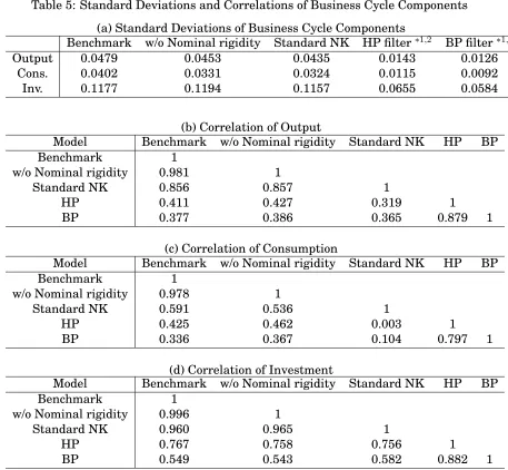
detrend the univariate time series2. Table 5 summarizes the standard deviations and
correlations of the business cycle components of these five approaches. Figures 2 and 3
also depict the decomposition of both trend and cycle components. The business cycle
components of output, consumption and investment in the models are defined asyˆt, ˆct
andˆit, and the trend component is defined asµAt .
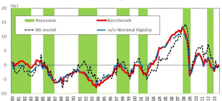
As can be seen from panel (a) of Figure 2, the cycle components of the output in the three DSGE models are highly aligned with one another, especially between the
bench-mark and the no nominal rigidity model. The second column of Table 5 (b) also shows
these high correlations. In addition, the peaks and troughs of these components seem to coincide with the recessions reported by the ESRI marked as green shaded areas. It
indicates that the business cycle components of the three DSGE models are successfully
extracted from the data. On the other hand, panel (b) depicts the common trend compo-nents of the real GDP in terms of the five approaches. While the trends of both the HP
and the BP filter pass through the center of the fluctuations of the actual GDP, those of
the DSGE model swing much higher and lower than the actual values in some periods. In particular, from 1984 to 1999, the trends locate upwards away from the real GDP,
2
whereas they locate downwards away from it during 2002 to 2007. These movements
are derived from big movements of the trend of investment, since the DSGE models impose the balanced growth theory between output and investment. According to the
DSGE models, the decline in R&D activities or TFP from 2002 to 2007 induces a huge drop in the common trend. As a result, exponential expansions of the business cycles are
observed in this period, as shown in panel (a).
The four panels of Figure 3 show the business cycle components of the real GDP, consumption and investment extracted from the benchmark model and the HP and BP
filters as well as the coincident business cycle index (CI) reported by the ESRI,
respec-tively. The blue solid lines marked with diamond symbols represent the cycles of the benchmark, while the red solid lines with asterisk symbols and the black dashed lines
are those extracted from the HP and BP filters, respectively. As can be seen from panels
(b) through (d), the peaks and troughs of the cycles of the three variables seem to match the recessions represented by the green shaded areas. As in panel (a), the fluctuations
of the three variables of the benchmark model are likely to be highly consistent with
those of the CI. Although the cycles of investment of the benchmark model are very sim-ilar to those of both the filters, the cycles of output and consumption extracted from the
DSGE model fluctuate much more than those of the filters. Again, these characteristic
movements are generated from the balanced growth theory working among the three macroeconomic variables. In contrast, both the filters independently extract the cycle
components by using only univariate information from each variable. These features,
such as the correlation among the five approaches, are also summarized in panels (b) through (d) in Table 5.
[ Insert Fig. 2 and Fig. 3 ]
[ Insert Table 5 ]
5.4 Variance and Historical Decompositions
5.4.1 Variance Decomposition Analysis
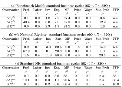
Justiniano, Primiceri and Tambalotti (2010) conducts unconditional variance decompo-sition regarding standard business cycle frequencies from 6 to 32 quarters. We follow
this approach and apply it to longer cycles including trend components regarding
fre-quency over 32 quarters in Table 6 in addition to the standard business cycles, as shown in Table 7. This analysis sheds light on the role of shocks in medium-term cycles as well
as short-term cycles.
the R&D success probability shock of the two DSGE models with endogenous growth
account for a much larger portion of the variances of the common trend than in the case of the cycle components for all three variables. For example, in the benchmark model,
the success probability shock contributes 29.4 % of the trend of output but only 3.6 % of the cycles of output. Surprisingly, in the case of the no nominal rigidity model, this shock
explains about 86.5 % of the trend of the output although only 14.0 % of the cycles. This
contrast between the two different frequencies might depend on the impact of the change in the R&D activities’ efficiency generated by the success probability shock. This change
influences the growth rate strongly but scarcely affects the business cycles. Similarly,
in the case of the standard NK model, the TFP shock contributes a larger ratio of the variances of the common trend than that of the cycles of all three variables. However,
the TFP shock accounts for large amounts of around 19 % to 68 % for all three variables
even in the short-term cycles. Accordingly, the success probability shock has different features from the TFP shock in both frequencies.
Second, the contribution of the monetary policy shock in the benchmark model is
very large in both frequencies regarding all three variables, as shown in Table 6 (a) and Table 7 (a). Similarly, the monetary policy shock accounts for a high percentage of
both trend and cycle components even in the standard NK model. These results stem
largely from the strong nominal rigidities suggested by the high Calvo price parameter, such as nearly 0.96, and the low price index parameter, such as 0.09. In other words,
the real variables are directly influenced by the monetary policy shock, since the price
level is hardly flexible. However, it is likely that the effect of the monetary policy is overestimated or includes a sort of upper bias, since the latter part of our sample period
includes the zero interest rate period. On the other hand, as shown in Table 7 (b), the
exogenous demand shock is a main contributor to the cycle components of the three variables in the no nominal rigidity model, since the Calvo price parameter is set to zero.
The monetary policy does not contribute to the variance of the real variables, as shown in panel (b) of Tables 6 and 7. Accordingly, the fluctuations in the real variables are
mainly explained by the real exogenous demand shock, instead of the monetary policy
shock, as a result of assuming the neutrality of money.
[ Insert Table 6 and Table 7 ]
5.4.2 Historical Decomposition Analysis
Before considering the historical decomposition, we mention the property of eight
struc-tural shocks. SincelogµA
key factor of economic growth,µAt, which can be rewritten as
logµAt = λx
1−αlog [ (1−δa) + ∆a,t(z
λ
t, ztb, zlt, zgt,ztP, ztW, zit, εRt ) ],
where µVt consists of the determined growth rate, (1−δa), and the stochastic growth
rate,∆a,t, which is generated from the combination of an additional goods variety. ∆a,t
is a sort of function that is affected directly by the R&D success probability shock zλt
and indirectly by the seven other shocks through the market mechanism. Hence, the
goods variety shock and the success rate shock have a permanent effect on the four series – output, consumption, investment and wage – via the R&D sector, whereas the
remaining shocks must also influence the common growth rate,µAt, through the change
in ∆a,t, although they have a tiny effect on the common growth rate, as shown in the
following figures.
Technology Progress Rate or Common Trend
Figure 4 shows the estimation and historical decomposition of the time series of the
common growth rate, µAt. Although the ranges of the rate after 1982:Q1 are located
between −1.5% and 1.5% in a quarterly period, most of the growth rates are shown
to have negative values between 1991:Q1 and 2013:Q1. These values might support
that period being referred to as the “lost decades.” Since we find two deep declines in
the progress rate during the Asian financial crisis in 1998 and the failure of Lehman Brothers in 2008:Q3, these two crises caused not only big recessions in terms of the
business cycle but also stagnation of the economic growth in terms of the supply side.
As shown in Figure 4, the historical decomposition of the common growth rate, µAt,
shows that the persistence of the positive R&D success rate shock (the area shaded in
blue) gradually increased the progress rate for the Plaza Accord3in 1985 before the
bub-ble boom started. However, the persistence of the negative R&D success rates dropped the growth rate by reducing a variety of new products after 1990:Q1. This shock also
decreased the common growth rate,µAt, after 1992:Q1. This figure suggests that a rise
(drop) in the R&D success rate induces expansion (shrinkage) of the variety of interme-diate goods. The activities of the R&D sector might positively affect the quantity of the
output in the productive sector via the fluctuation of converting innovation into
interme-diate goods variety. Furthermore, sluggish spending of the R&D investment shrunk the variety of new products in the productive sector, and then both the R&D investment and
3
the variety of new products fell by feeding on each other.
After 1997 the stagnation can mainly be explained by the persistent declines in the R&D success rate shock. This might also be regarded as reductions in R&D investment
attributed to the financial problems of the corporate sector, although our model does not include the financial sector.
On the other hand, the labor disutility, monetary policy and price markup shocks
have very tiny but positive effects on the growth rate, whereas the exogenous demand shock, including the government spending policy, does not affect the growth in the
sam-ple period overall.
[ Insert Fig. 4 ]
Cycle Components of GDP, Consumption and Investment
Next we consider the decomposition of the business cycle components of output,
con-sumption and investment, defined asyˆt,ˆct andˆit, as shown in panels (a) through (c) of
Figure 5, respectively. The investment efficiency, labor disutility and exogenous
spend-ing shocks affect the three cycle components in the same direction, while the preference
and R&D success rates must have a contrasting effect on investment and consumption with the opposite direction via the substitution effect between consumption and saving.
We consider two shocks, namely the R&D success rate and preference shocks, which
have a substitution effect. The former positive shock increased the cycle of investment as well as the common trend until 1991, that is, the end of the ”bubble boom,” and then
the negative shock decreased the cycle after the end of the boom, as shown in Figure
5 (c). This shock, however, had opposite effects on the cycles of consumption, as shown in Figure 5 (b). On the other hand, the latter negative shock sustained a certain level
and decreased the consumption after 1991, as presented in Figure 5. This negative
preference shock increased investment and induced upward pressure on the output for that period, as shown in Panel (c).
To sum up, the fluctuation in the R&D success rate exerted a strong impact on the long stagnation in the three cycles after the ”bubble boom”, as shown in the three
pan-els. Again, if we regard the R&D success rate as R&D investment, a reduction in R&D
investment also caused a drop of a large fraction of physical investment. However, this reduction contributed to an increase in consumption due to the lower level of the nominal
interest rate.
Inflation
Panel (d) in Figure 5 depicts the decomposition of inflation. Although the contribution to
inflation is mainly accounted for by the price markup shock and the labor supply shock, the former pulls it downwards and the latter pushes it upwards. Since 1994 a reduction
in the success rate of the R&D sector has decreased inflation. The effect of the monetary
policy shock is not observed at all.
Labor Supply
Panel (e) in Figure 5 shows the decomposition of the labor supply. As shown in the figure,
the labor disutility and preference shocks in addition to the R&D success rate shock are the main sources of variations in the labor supply. Although the successive decline of
labor hours after 1990 is explained by the series of negative labor shocks in our model,
we are strongly convinced that a drastic change of social institutions and environments actually happened and attacked households, and this must be a factor in the deep decline
of the labor supply.
6
Conclusion
In this paper, following Comin and Gertler (2006), we incorporate the endogenous
pro-ductivity growth framework of Romer (1990) into a medium-scale new Keynesian DSGE model with nominal price and wage rigidities to evaluate the Japanese economy after
1980 for over three decades, including the bubble burst in 1991, the Asian currency
cri-sis in 1998 and the Lehman Brothers’ failure in 2008. To measure the performance of our DSGE model, we also build two alternative models, specifically one that excludes
the assumption of nominal rigidities and another that is a standard DSGE model with
an exogenous TFP shock. Using Bayesian estimation, we decompose the original time series into business cycles and the trend and compare them with those extracted by the
HP and BP filters. We find the factors that contributed to the huge declines in output
during the three economic crises by calculating the historical decomposition of the trend. The contributions of this study are twofold. First, we estimate a DSGE model with
the framework of R&D endogenous growth proposed by Comin and Gertler (2006) for
Japan. In addition, we evaluate this model by implementing the model selection out of the three models. Second, we introduce a new structural shock regarding R&D activities.
In terms of the new R&D shock as well as standard DSGE shocks, we empirically classify
We empirically find that, for Japan, the standard NK model with the TFP shock is
superior to our models with the endogenous growth model, regardless of the presence or absence of nominal rigidities. However, limiting the model selection to the two
en-dogenous growth models, the assumption of nominal rigidities of prices and wages is important to explain the data for over three decades. Furthermore, the R&D activity
and investment shocks account for the larger portions of the business cycle components
of the real GDP and investment. Furthermore, the common trends of the three DSGE models fluctuate with much greater volatility than those of both the HP and BP filters.
Finally, we observe that the two deep declines in the R&D activities during the Asian
financial crisis in 1998 and the Lehman Brothers’ failure in 2008:Q3 produced not only big recessions in the business cycles but also stagnation of the economic growth.
A
Appendix
A.1 Structural equations of the NK model with endogenous growth
A.1.1 R&D sector
Innovators
1. Innovation accumulation (R&D investment) from Eq.(1):
1
at
= 1−δz
µt
1
at−1
+φtid,t.
2. Efficiency of R&D investment from Eq.(2):
φt=
χz
at−1 i1d,t−ρ
.
3. No-arbitrage condition for innovation from Eq.(3).
id,t= (1−δz)µAt
1
at
− 1−δz
µVt at−1
EtΛt|t+1 jt+1.
Adopters
1. Success probability from innovation to new product from Eq.(6):
2. Technology progress rate from Eq.(7):
µAt = µVt 1λx−α.
3. Newly adopted innovation from Eq.(8):
˜
∆a,t= (1−δa)
1
at−1
−1
λt.
4. FOC of adopted innovation from Eq.(9):
ia,t= (1−δa) ωa λt
pVt − µ
A t
µV t
EtΛt|t+1 jt+1
.
5. Value of unadopted innovation from Eq.(10):
jt= (1−δa)
(1−ωa)λtpVt +{1−(1−ωa)λt}
µA t
µV t
EtΛt|t+1jt+1
.
A.1.2 Productive sector
Wholesaler
1. Marginal cost of wholesaler from Eq.(17) and (32):
mct= (1 +λx)st.
2. Price version of New Keynesian Philips Curve (NKPC) 1 from Eq.(19):
πto πt
= (1 +λpztp)k
p t
ftp.
3. Price version of NKPC 2 from Eq. (20):
ktp = mctyt+ξpEtµAt Λt|t+1
πγp
t π1−γp
πt+1
−1+λpλp kpt+1.
4. Price version of NKPC 3 from Eq. (21):
ftp =yt+ξpEtµAt Λt|t+1
πγp
t π1−γp
πt+1
−
1
5. Price version of NKPC 4 from Eq. (22):
1 =ξp
πγp
t−1π1−γp
πt
!−λp1
+ (1−ξp)
πto πt
−λp1 .
Intermediate Goods Firms
1. Implemented technology (goods variety) accumulation from Eq.(29) :
µVt = 1−δa+
(
1−Sa ∆˜a,t
˜ ∆a,t−1
µV t−1
µV
!)
˜ ∆a,t.
2. Capital depreciation rate function from Eq.(27):
δukt=δk+bk
ukt1+ζk
1 +ζk
.
3. Marginal capital depreciation rate from Eq.(27) :
δ′ukt=bk
uktζk.
4. Marginal productivity of capital stock from Eq.(33) :
rtk=αst
µAt−1yt
uk tkt−1
.
5. Marginal productivity of labor from Eq.(34) :
wt= (1−α)st
yt
lt
.
6. Realized technology price from Eq.(35) :
pV t =γta
n
1−Sa
∆˜ a,t
˜ ∆a,t−1
µV t−1 µV
−S′
a
∆˜ a,t
˜ ∆a,t−1
µV t−1 µV ˜ ∆a,t ˜ ∆a,t−1
µV t−1 µV
o
+µVΛ
t|t+1γta+1Sa′
∆˜ a,t+1 ˜ ∆a,t µV t µV ˜ ∆a,t+1
˜ ∆a,t µV t µV .2
7. Goods variety adjusment cost function:
Sa
˜ ∆a,t
˜ ∆a,t−1
µVt−1 µV ! = 1 2 1 ζa ˜ ∆a,t ˜ ∆a,t−1
µVt−1 µV −1
8. Derived Goods variety adjusment cost function:
Sa′ ∆˜a,t
˜ ∆a,t−1
µV t−1
µV
!
= 1
ζa
˜ ∆a,t
˜ ∆a,t−1
µV t−1
µV −1
! .
9. Tobin’s Q of goods variety Eq.(36):
γa,t
µVt µA
t
=EtΛt|t+1{(1−δa)γa,t+1+λxst+1yt+1}.
10. Production function from Eq.(26):
yt=
uk tkt−1
µA t−1
!α l1t−α.
A.1.3 Households
1. Marginal utility of consumption from Eq.(40):
λct= µ
A t−1zbt
µA
t−1ct−hct−1
−β hEt
ztb+1 µA
tct+1−hct
.
2. Stochastic discount factor (SDF) from Eq.(41):
µAtΛt|t+1 =βEt
λct+1 λct .
3. Euler equation from Eq.(42):
Λt|t+1= Et
πt+1
rnt .
4. Fixed capital accumulation from Eq.(28):
kt=
n
1−δukto kt−1 µAt−1 +z
i t
(
1−S it it−1
µAt−1 µA
!) it.
5. FOC with respect to capital utilization rate from Eq.(45):