Munich Personal RePEc Archive
Monetary Policy in a Small Open
Economy with Non-Separable
Government Spending
Troug, Haytem
University of Exeter
2 March 2019
Monetary Policy in a Small Open Economy with
Non-Separable Government Spending
Haytem Troug
∗March 3, 2019
Abstract
To show how fiscal policy affects the transmission mechanism of monetary policy, we
ex-tend a standard new Keynesian model for a small open economy to allow for the presence
of non-separable government consumption in the utility function. We show how monetary
policy should optimally respond to demand and supply shocks when the government
sec-tor is incorporated into the model. The introduction of government consumption affects the
transmission of monetary policy. When government consumption has a crowding in effect on
private consumption, it will dampen the transmission mechanism of monetary policy, and vice
versa. Nevertheless, the degree of openness will minimise the effect of the introduction of
government consumption in a non-separable form. Data for 35 OECD countries empirically
support these findings, and the empirical results are robust to the zero lower bound period.
The theoretical model also shows that, once we model the rest of the world economy, domestic
government consumption and foreign government consumption will have opposing effects on
private consumption, which contradicts with the existing literature.
Keywords: New Keynesian models, Business Cycle, Monetary Policy, Open Economy
Macroeco-nomics, Joint Analysis of Fiscal and Monetary Policy.
JEL classification: E12, E32, E52, E63, F41.
∗University of Exeter Business School, Department of Economics, Streatham Court, Rennes Drive, Exeter, EX4
1
Introduction
The substantial role of government consumption in influencing economic activity raises the
ne-cessity for monetary policy to take into account the behaviour of fiscal policy and to also take
into account how the presence of the fiscal sector affects the transmission mechanism of
mone-tary policy. Despite being a flexible tool that can address several macroeconomic issues, DSGE
models have been rarely used to analyse the interaction between monetary and fiscal policy until
the post-financial crisis. The recent literature (see, e.g.,Christiano et al. 2011;Davig and Leeper
2011) focused on the impact of fiscal policy only when monetary policy is constrained by the
zero-lower-bound, leaving a gap in the analysis of how governemnt consumption affects the transmission
mechanism of monetary policy1. That motivates this paper to analyse how government
consump-tion affects the dynamics of a small open economy, once the former is included in a non-separable
form to the utility function. To the best of our knowledge, this issue has not been addressed by
the literature, and we aim to do so in this paper.
The standard hypothesis of DSGE models introduces government consumption as either
com-plete waste (Obstfeld and Rogoff 1995; 1996) or included in preferences in a non-separable form.
While the former became an obsolete assumption in the recent literature, the inclusion of
govern-ment consumption to preferences in a separable form was adopted both in New Keynesian models
(Smets and Wouters 2007 and Gali and Monacelli 2008) and in RBC models (Baxter and King
1993). Despite being understudied, as noted by Cantore et al. 2014, the inclusion of government
consumption seems appealing, given that agents gain utility from government consumption and the
purpose of the government delivering services to households supports this claim. However,
assum-ing prior separability in preferences between private consumption and government consumption
can produce biased estimates of the response of private consumption, labour supply, and, hence,
of output to a government consumption shock, as recently highlighted byErcolani and Azevedo
2014.
Gali, Lopez-Salido, et al. 2007challenged the adverse effect of government consumption on
pri-vate consumption produced by these DSGE models. They highlighted the discrepancy between the
1Following the work of Troug 2019, we use the term "government consumption" in this paper for non-fixed
estimates of these DSGE models and the ones produced by some empirical models which illustrate
a positive effect of government consumption on private consumption. Bouakez and Rebei 2007and
Pieschacon 2012, among others, have also supported the complementarity assumption between
pri-vate consumption and government consumption. The two papers employ an RBC model and use
the complementarity assumption to analyse the effect of a government consumption shock on the
economy. Nevertheless,Ercolani and Azevedo 2014showed results that indicate that government
consumption is a substitute for private consumption in a New Keynesian framework. Ganelli 2003
also introduced government consumption as a substitute for private consumption. The elasticity of
substitution between government consumption and private consumption in Ganelli’s model governs
how much private consumption needs to decline in response to an increase in government
consump-tion in order to hold the utility on the same indifference curve. The discrepancy in the literature
goes beyond the theoretical models, where even empirical models illustrate different estimates for
the effect of government consumption, which depend on the modelled time frame and the adopted
estimation method2.
The above complications raise a crucial question regarding the reaction of monetary policy
to different shocks once government consumption is included to the utility function in a
non-separable form. Once government consumption is included in a non-non-separable form, it will affect the
marginal utility of consumption and consequently the labour supply condition and the consumption
smoothing condition. As a result, this inclusion will affect the structure of the whole model, and
the transmission mechanism of monetary policy. As noted above, the existing literature has not
addressed this issue, and we aim to fill in this gap in this paper. The mechanism of this model
applies to both the complementarity case and the substitutability case, and we will focus on changes
in the reaction and the transmission mechanism of monetary policy once government consumption
is incorporated to a standard New Keynesian model in a non-separable form.
This paper employs a New Keynesian model to study the optimal response of monetary policy
to supply and demand shocks in the presence of fiscal policy for a small open economy. To do
this, we extend an otherwise standard New Keynesian model for a small open economy (Galí
and Monacelli 2005) and build from the model used in Troug 2019 to allow for meaningful
non-2
separable government consumption, financed by means of lump-sum taxes, in the utility function.
Extending the model to a small open economy case complicates the problem for monetary policy to
the extent that the authorities must additionally take into account how the exchange rate affects
other macroeconomic variables. Similar to the closed-economy case, we are able to derive an
optimal monetary policy rule which takes into account developments in government consumption,
in addition to developments in the rest of the world economy. The other extension that this paper
adds to the canonical small open economy model is modelling the rest of the world economy as an
aggregate of identical small open economies, and each of them has a size of zero, following the work
ofUnalmis et al. 2008. This will allow us to trace the spillover effects of supply and demand shocks
in the foreign economy on the domestic economy. I choose this framework over the two-country
model, adopted in (Obstfeld and Rogoff 1995; 1996) andGanelli 2003, to prevent spillovers from
the domestic economy to the rest of the world economy that might complicate the analysis.
In the open-economy case, the degree of openness will minimise the deviation of the slope of
the IS curve from the standard case both in the complementarity and the substitutability case.
Moreover, the degree of openness minimises the crowding-out (-in) effect of government
consump-tion on monetary policy when the former is a complement (substitute) to private consumpconsump-tion.
We also find that the fiscal multiplier is also minimised by the degree of openness of the economy,
in comparison to the closed-economy version of the model. We additionally find that the size of
the fiscal multiplier is negatively affected by the response of monetary policy and the flexibility of
the exchange rate, which is in line with the theoretical findings of, among others,Woodford 2011,
and the empirical results ofKoh 2017and contradicts with the findings ofTroug 2019.
Moreover, in the case of the spillover effect of external shocks, the amount of exchange rate
volatility will determine how much the domestic economy will be affected by external shocks. In
this regard, we find that the main difference in the dynamics between this model and the one
used inGanelli 2003is the exchange rate channel in the two models. In this model, the exchange
rate is a product of the interest rates differentials, and the purchasing power of the domestic
consumers will be affected by any changes in the exchange rate. On the other hand, in Ganelli’s
model, the exchange rate is a function of the money demand, which is, in return, a function of
private consumption and government consumption. This difference in the dynamics between the
on domestic private consumption in our model, while the two have the same adverse effect on
domestic consumption in Ganelli’s model.
The empirical results of this paper support the findings of the theoretical model. First, the
results show that government consumption in 35 OECD countries has a crowding in effect on private
consumption. Second, this positive effect of government consumption dampens the negative effect
of the policy rule on private consumption. Nevertheless, the degree of openness in the economy,
measured as net exports as a ratio of output, minimises the crowding out effect of fiscal policy on
monetary policy. These results are robust to the zero lower bound period.
The remainder of the paper is organised as follows. We will first demonstrate the structure of
our model in the second section. In the third section, we show the parametrisation of the model.
The equilibrium dynamics of the model will be discussed in the fourth section. The analysis of
the impulse response functions is presented in the fifth section. In the sixth section, we show the
results of the welfare loss calculations and the second moments of the primary variables of the
small open economy. Lastly, the concluding remarks will take place in the seventh section.
2
Small open economy model
32.1
Households in the domestic economy
Our economy is populated by a representative household that derives utility from aggregate
con-sumption and leisure. The household is assumed to live infinitely and in each period is endowed
with one unit of time that is divided between work and leisure: Nt+Lt= 1. The representative
consumer seeks to maximise the following discounted lifetime utility function:
E0
∞
X
t=0
βtU( ¯C
t, Nt) (1)
The utility function is assumed to be continuous and twice differentiable. Where Nt is the
number of hours worked; β is the discount factor; ¯Ct is the aggregate consumption bundle. The
aggregate consumption bundle is a constant elasticity of substitution that consists of private
con-3 We will only display the model for the small open economy in the main body of this paper. We show the
sumptionCtand government consumptionGt4:
¯
Ct=
h
δχC1−χ
t + (1−δ)χG
1−χ t
i1−1χ
(2)
Where δ is the share of private consumption in the aggregate consumption bundle and χ is the inverse elasticity of substitution between private consumption and government consumption.
Equations (1) and (2) show that the utility function is non-decreasing in government consumption
Gt. The above utility function is subject to the following budget constraint:
Z 1 0
PH,t(j)CHt(j)dj+
Z 1 0
Z 1 0
Pi,t(j)Cit(j)djdi+EtQt,t+1Dt+1≤Dt+WtNt+Tt (3)
WhereDtis the nominal payoff at period t+1 of bonds held at the end of period t including shares
in firms, government bonds, and different types of deposits. Qt,t+1 is a stochastic discount factor
of nominal payoffs and it is equal toR1t;Wtis the wage;Ttis lump-sum transfers to the households
net of lump-sum taxes. All units are expressed in terms of domestic currency.
The utility function that we use assumes two separabilities. The first one is the separation
between consumption and the amount of hours worked, and the second one is time separability.
The household’s problem is also analysed in two stages here: we first deal with the expenditure
minimisation problem faced by the representative household to derive the demand functions for
domestic and foreign goods. In the second stage, the households choose the level ofCt and Nt,
given the optimally chosen combination of goods. Ctis our basic private consumption bundle, and
it is a CES composite of home and foreign goods defined as follows:
Ct=
h
(1−α)1ηC η−1
η
H,t + (α)
1
ηC η−1
η
F,t
iη−η1
(4)
The above equation is the same household consumption bundle used by Galí and Monacelli
2005, which is the workhorse for small open economies. αhere is the degree of openness in the
4Government consumption in this framework can be thought of as a public good that households consume at
economy which represents the share of imported goodsCF,tin the household’s consumption bundle.
Conversely, the home bias parameter (1−α) produces the possibility of a different consumption bundle in each economy. This is a consequence of having different consumption baskets in each
country, despite the law of one price holding for each individual good. η > 0 is the elasticity of substitution between domestically produced goods and imported goods in the household’s
con-sumption bundle. Concon-sumption goods that are produced either at home or in any foreign country
are represented by the unit interval: Cj,t =
R1 0 Cj,t(i)
ǫ−1
ǫ difori∈[0,1] andj = [H, F, i∈[0,1]]. Now as a first step, the households must minimise their expenditure by optimally choosing the
share of each good in the aggregate consumption bundle. Doing so will yield the following demand
functions:
Ci,t(j) =
Pi,t(j)
Pi,t
−ǫ
Ci,t, CH,t(j) =
PH,t(j)
PH,t
−ǫ
CH,t, Ci,t=
Pi,t
PF,t
−γ
CF,t (5)
WherePi,t≡(R
1 0 Pi,t(j)
1−ǫdj)1−ǫis the aggregate price index for imported goods from country
(i),PH,t ≡(
R1 0 PH,t(j)
1−ǫdj)1−ǫ is the aggregate price index for domestic goods, and P
F,t is the
aggregate price index for imported goods. The first two terms show domestic demand for good (j)
in one of the foreign economies and in the home economy, respectively. The parameterǫrepresents how much the demand for good (j) will decline if the relative price of that good increased by 1 unit.
A lower elasticity of substitution indicates higher consumption of the good of interest. This shows
that the goods in the consumption bundle are not perfect substitutes. The third equality is domestic
demand for goods produced in country (i) as a function of total domestic demand for foreign goods, andγ > 0 is the elasticity of substitution between goods from different origins. We finally show the demand functions of domestic and foreign goods from their expenditure minimisation given
total consumption:
CH,t= (1−α)
PH,t
Pt
−η
Ct; CF,t=α
PF,t
Pt
−η
Ct (6)
Now we turn our attention to the per-period utility function in the following form5:
5We replaced private consumption in the utility function with the aggregate consumption bundle. As noted
U(Ct, Nt;Gt) =
¯
Ct1−σ−1
1−σ − Nt1+ϕ
1 +ϕ, (7)
Whereσis the inverse elasticity of intertemporal substitution. Settingσequal to 1 implies that the household has a log-utility in consumption; ϕ is the inverse Frisch labour supply coefficient, andϕ >0 also measures the curvature of the marginal disutility of labour. The above equation is subject to the aggregate budget constraint, which we get by plugging the above demand bundles
and price indices in equation (3):
PtCt+Et[Qt,t+1Dt+1]≤Dt+WtNt+Tt (8)
WhereEt is the conditional expectations operator. The household’s total expenditure basket
is equal to: PtCt =R
1
0 PH,t(j)CHt(j)dj+
R1 0
R1
0 Pi,t(j)Cit(j)djdi. Pt is the consumer price index (CPI) and it is equal to: Pt=
h
(1−α)(PH,t)1−η+α(PF,t)1−η
i1−1η
. From Equation (7) and (8) we
can write the standard optimality condition for households as follows:
Wt
Pt
=NtϕC¯tσ
Ct
¯
Ct
χ
δ−χ (9)
The intertemporal optimality condition is:
βC¯t¯+1 Ct
χ−σ Pt
Pt+1 Ct
Ct+1 χ
=Qt,t+1 (10)
Taking the conditional expectation of equation (10) and rearranging the terms we get:
βRtEt
hC¯t+1
¯
Ct
χ−σ Pt
Pt+1 Ct
Ct+1 χi
= 1 (11)
WhereRt=Et(Q1t,t+1) is the one-period return from a riskless bond andQt,t+1is the price of that
bond. Equations (9) and (11) deviate from the standard open economy literature. This deviation
is due to the fact that we have included government consumption in the aggregate CES basket
with private consumption in a non-separable form. The first equation depicts the labour supply
dynamics. It shows labour supply as a function of the real wage given the aggregate consumption
on labour supply depends on the value ofχ. Noting that in the Cobb-Douglas case, whenχ=σ, the labour supply equation collapses to its canonical form as government consumption would have
no effect on private consumption. When χ > σ, government consumption will have a negative effect on real wages given its positive effect on labour supply. On the other hand whenχ < σ, government consumption will have a positive effect on real wages, resulting from its negative effect
on labour supply. The second equation is the Euler equation which characterises consumption
smoothing. The Euler equation in this model also deviates from the standard form found in the
literature. In this case, the smoothing of the aggregate consumption bundle ¯C is included in the above Euler equation. In the Cobb-Douglas case, when χ = σ, the above equation would also collapse to the canonical version of the Euler equation. Whenχ > σ, changes in the current value of the aggregate consumption bundle will have a positive effect on private consumption. However,
the aggregate consumption bundle will have an adverse effect on private consumption whenχ < σ.
2.2
Firms
2.2.1 Price Setting Behaviour
The firms in this model set their prices in a staggered way followingCalvo 19836. Under Calvo
contracts, we have a random fraction 1−θ of firms that can reset their prices at periodt, while the remaining firms of sizeθkeep their prices fixed at the previous period’s price level. Therefore, we can say thatθk is the probability that a price set at periodtwill still be valid at period t+k.
Thus, the probability of a firm re-optimising its prices will be independent of the time elapsed since
it last re-optimised its prices, and the average duration for prices not to change is 1
1−θ. Given the
above information, the aggregate domestic price level will have the following form:
PH,t=
h
θ(PH,t−1)1−ǫ+ (1−θ)( ¯PH,t1−ǫ)
i1−1ǫ
(12)
Where ¯PH,t is the new price set by the optimising firms. From the derivations shown in
Appendix 2, we get the following form for inflation:
6The Calvo model makes aggregation easier because it gets rid of the heterogeneity in the economy. The
Π1−ǫ
H,t =θ+ (1−θ)
P¯H,t
Pt−1 1−ǫ
(13)
The above equation shows that the inflation rate at any given period will be solely determined
by the fraction of firms that reset their prices at that period. When a given firm in the economy sets
its prices, it seeks to maximise the expected discounted value of its stream of profits, conditional
that the price it sets remains valid:
maxP¯H,t
∞
X
k=0
θkEtQt,t+k[cjt+k|t( ¯PH,t−Ψt+k)] (14)
The above equation is subject to a sequence of demand constraints: cjt+k =
P¯H,t
PH,t+k
−ǫ
Ct.
Solving this problem (also shown inAppendix 2) yields the following optimal decision rule:
∞
X
k=0
θkE t
n
Qt,t+kCt+k
h P¯H,t
PH,t−1
− MM Ct+k|tΠHt−1,t+k
io
= 0 (15)
Where M is the firm’s price markup at the steady state and M Ct is the real marginal cost
that firms face in the domestic economy. As we can see from equation (15), in the sticky price
scheme producers, given their forward-looking behaviour, adjust their prices at a random period
to maximise the expected discounted value of their profits at that period and in the future. Thus,
firms in this model will set their prices to equal a price markup plus the present value of the future
expected stream of their marginal costs. This is done because firms know that the price they set
at periodt will remain valid for a random period of time in the future. We also assume that all firms in the economy face the same marginal cost, given the constant return to scale assumption
imposed on the model and the subsidy that the government pays to firms, as we will see in the
following section. The firms also use the same discount factorβ as the one used by households, and this is attributed to the fact that the households are the shareholders of these firms. Also,
all the firms that optimise their prices in any given period will choose the same price, and this is
also a consequence of the firms facing the same marginal cost. Equation (15) also shows that the
inflation rate is proportional to the discounted sum of the future real marginal costs additional to
2.2.2 Production
Firm (j) in the domestic economy produces a differentiated good following a linear production function:
Yt(j) =AtNt(j) (16)
WhereYt(j) is the output of final good (j) in the domestic economy. Atis the level of technology
in the production function, and it is assumed to be common across all firms in the economy and
exogenously evolves. Nt(j) is the labour force employed by firm (j). The log form of total factor
productivityat=log(At) is assumed to follows an AR(1) process: at=ρaat−1+ǫa,t. 0< ρa >1
is the autocorrelation of the shock, and the innovation to technologyǫa,t has a zero mean and a
finite varianceσa. We exclude capital from production in this model for the sake of tractability.
Aggregate output and aggregate employment in the domestic economy are defined by the Dixit
and Stiglitz 1977aggregator:
Yt=
Z 1 0
Yt(j)
ǫ−1
ǫ dj
ǫ−ǫ1
;Nt=
Z 1 0
Nt(j)
ǫ−1
ǫ dj
ǫ−ǫ1
(17)
Given the common technology assumption across all firms of the economy, the total cost function
for firm (j) is defined as follows:
T Ct(j) =
(1−τ)WtYt(j)
At
(18)
In the above equation, we leftWtwithout any firm specification, which is attributed to the fact
that we have a competitive labour market. Also, τ is the subsidy that the government gives to firms in order to eliminate the markup distortion created by the firms’ monopolistic power. Taking
the first order condition of equation (18), with respect to production, yields the following marginal
cost equation:
M Ct(j) =
(1−τ)Wt
At
(19)
From the above equation, it is clear that the constant return to scale assumption makes the
across all firms: M Ct(j) =M Ct. Now the common real marginal cost will look like:
M Cr t =
(1−τ)
At
Wt
PH,t
(20)
The marginal cost equation is expressed in terms of the domestic prices levelPH,t, wages Wt,
total factor productivityAt and τ, which is the subsidy that the government gives to firms, in
order to eliminate the markup distortion created by the firms’ monopolistic power.
Lastly, after the aggregation of output and employment, we get the following aggregate
pro-duction function:
Yt=AtNt (21)
2.3
International Linkages
We first start by the defining the terms of trade as the ratio of imported prices to domestic prices.
The bilateral terms of trade between the domestic economy and another small economy (country i)
is defined as: Si,t =PPH,ti,t. Thus, the aggregate terms of trade is defined as: St=
R1 0 S
1−γ i,t di
1−1γ .
DefiningPF,t=
R1 0 P
1−γ i,t di
1−1γ
allows us to define the aggregate effective terms of trade as:
St=
PF,t
PH,t
(22)
If we plug in the log-linearised representation of the imported prices index from the above
equation (pF,t =st+pH,t) in the log-linearised form of the CPI price index equation, we will be
able to derive the CPI index as a function of the domestic prices index and the terms of trade:
pt=pH,t+αst (23)
The above function shows that a gap exists between the CPI index and the domestic price index
which is filled with the terms of trade. The gap is parametrised by the degree of openness of the
domestic economy. Before progressing to further derivations, we first define the bilateral exchange
rateEi,t as the value of country i’s currency in terms of the domestic currency. Assuming that the
Pi,t(j) =Ei,tPi,ti (j) (24)
Integrating the above equation yields the price index for country (i). Solving this integrate for
the imported prices index in the domestic economy yields:
PF,t=EtPt∗ (25)
The nominal effective exchange rate is equal to Et ≡ R01Ei,tdi, and the world price index
is defined as P∗
t ≡
R1
0 Pi,tdi. Plugging the value of the imported prices index from the above
equation in the definition of the terms of trade yields:
St=
EtPt∗
PH,t
(26)
We now define the bilateral real exchange rate as the ratio of the price index in country (i)
to the CPI index in the domestic economy: REERi,t = Ei,tP
i t
Pt . Integrating the bilateral real exchange rate equation yields the real effective exchange rate equation for the domestic economy:
REERt =
EtPt∗
Pt . From the definitions of the terms of trade and the real effective exchange rate, we can define the equation that links the two variables in a log-linearised form as follows:
qt= (1−α)st (27)
Under the assumption of complete international financial markets, the price of a one-period
riskless bond from country (i) dominated in the domestic economy’s currency is equal to: Ei,tQit=
E[Ei,t+1Qt,t+1]. If we add this equation to the domestic bond’s price equation (Qt=E[Qt,t+1]),
we get the uncovered interest rate parity condition:
Qi t
Qt
=Et
Ei,t+1 Ei,t
(28)
The uncovered interest parity condition is crucial for the no-arbitrage condition to hold in the
perfect substitutes for domestic bonds once both of them are expressed in the same currency. The
uncovered interest parity equation also implies that higher foreign interest rates or depreciation in
the exchange rate will put upward pressure on domestic interest rates.
The last thing that we need do in this section is to derive the international risk condition. Under
the assumptions of complete international markets and the identical preferences assumption, the
foreign consumer’s Euler equation can be transformed to:
βC¯
∗
t+1
¯
C∗
t
χ−σ P∗
t P∗ t+1 C∗ t C∗ t+1
χ Et Et+1
=Qt,t+1 (29)
We then divide the domestic inter-temporal optimality condition (eq. 10) by the foreign
econ-omy’s inter-temporal optimality condition (eq. 29) to get:
1 =Et
C¯t+1 ¯
Ct
χ−σ
Pt
Pt+1
Ct
Ct+1
χ C¯∗
t+1
¯
C∗
t
χ−σ P∗
t
P∗
t+1
Et Et+1
C∗ t C∗ t+1 χ ! (30)
Plugging the definition of the real effective exchange rate in the above equation yields:
Ct=VtCt∗(REERt)
1
χ
C¯t
¯
C∗
t
χ−χσ
(31)
Where Vt = Ct+1
¯
C
∗χ−σ
χ t
C∗
t+1C¯
χ−σ χ t+1 REER
1
χ t+1
is a constant which depends on the initial relative wealth
position. We assume that we have a symmetric initial condition and setVt = 1, meaning that
the net position of foreign assets is equal to zero. Thus, the international risk sharing condition
simplifies to:
Ct=Ct∗(REERt)
1
χ
C¯t
¯
C∗
t
χ−χσ
(32)
Complete security markets ensure that risk-averse consumers can trade away the risks and
the shocks they encounter. Under this setting, consumers can purchase contingent claims for
realisations of all idiosyncratic shocks, and this will enable them to diversify all idiosyncratic risk
through the capital markets. Also, the above international risk sharing condition depicts how a
depreciation in the real effective exchange rate would boost domestic consumption relative to the
condition is:
ct=c∗t+
(σ−σδ)
σδ
(g∗t −gt) +
1
σδ
qt. (33)
Whereσδ =δσ+ (1−δ)χ is a weighted average of the intertemporal elasticity of substitution
σ and the inverse elasticity of substitution between government consumption and private con-sumptionχ. The above equation illustrates how the effect of domestic and foreign government consumption is governed byχ. In the Cobb-Douglas case whenχ=σ, the above international risk sharing condition collapses back to its standard representation asσδ =σ. In this case, government
consumption both in the domestic and foreign economy will not affect private domestic
consump-tion. Whenχ > σ, domestic government consumption has a positive effect on private consumption, while foreign government consumption has a negative effect on domestic private consumption. On
the other hand, when χ > σ domestic government consumption will have a negative effect on private consumption and foreign government consumption will have a positive effect on private
consumption. This last point makes a clear distinction between our model and the one used in
Ganelli 2003. Where in the latter’s both domestic and foreign government consumption have the
same negative effect on private consumption. In this setting, as will be made clear in the
simu-lations below, monetary policy will react to changes in government consumption, conditional on
how government consumption affects the economy. The exchange rate will react to the movement
in the interest rates differential affecting the purchasing power of domestic private consumers.
2.4
Market Clearing Conditions
We start by identifying the market clearing condition for the domestically produced products in
the small open economy. Where domestic output of good (j) is absorbed both by domestic demand
and foreign demand:
Yt(j) =CH,t(j) +
Z 1 0
Ci
H,t(j)di (34)
In the above equation,CH,t(j) is domestic demand for good (j) andCH,ti is country (i)’s demand
for good (j) in the domestic economy. We plug the domestic demand function for good (j) (eq.5).
across all the countries of the world economy to get:
Ci H,t(j) =
PH,t(j)
PH,t
−ǫ PH,t Ei,tPF,ti
−γPF,ti
Pi t
−η
(35)
Plugging in the respective demand bundles transforms the market clearing condition for
do-mestic production of good (j) to:
Yt(j) =
PH,t(j)
PH,t
−ǫ
(1−α)PH,t
Pi t
−η
Ct+α
Z 1
0
PH,t Ei,tPF,ti
−γPF,ti
Pi t
−η
Cti(j)di
(36)
Using the Dixit-Stiglitz aggregater of domestic output, we can write the above equation in
aggregate terms:
Yt=
PH,t
Pi t
−η
(1−α)Ct+α
Z 1
0
Ei,tPF,ti
PH,t
γ−η
Qηi,tCi tdi
(37)
In the above equation, we tookPH,t
Pi t
−η
as common factor. We have also used the definition
of the bilateral real exchange rate. If we divide and multiply the termEi,tPF,ti
PH,t
γ−η
by Pi,t we
get: Pi,t
PH,t Ei,tPF,ti
Pi,t
γ−η
. The two terms that we get are essentially the effective terms of trade for
country (i) and the bilateral terms of trade between the domestic economy and country (i), and
equation (37) simplifies to:
Yt=
PH,t
Pi t
−η
(1−α)Ct+α
Z 1 0
Si tSi, t
γ−η
Qηi,tCi tdi
(38)
Taking the first order log-linearisation of the above equation around a symmetric steady state
yields:
yt= (1−α)ct+αc∗t+α[γ+η(1−α)]st (39)
Adding the international risk sharing condition to the above equation yields:
yt=y∗t +
(1−α)(σ−σδ)
σδ
(gt∗−gt) +
ωα
σδ
st (40)
where ω =σδγ+ (1−α)(ησδ−1) and ωα = (1−α) +αω. The above equation links actual
terms of trade. From the above equation, we notice that the terms of trade variable is the only
channel through which monetary policy could have an effect on the actual rate of output. In this
regard, the monetary policy rule will be adjusted to achieve the required movement in the terms
of trade to close the output gap.
2.4.1 The Supply Side of the Economy
The equation of the natural rate of output (derived inAppendix 1) takes the following form:
¯
yt=
ωα(1 +ϕ)
ωαϕ+σδ
at+
σδ(ωα−1)
ωαϕ+σδ
y∗t−αω(σ−σδ)
ωαϕ+σδ
gt∗−(1−α)(σ−σδ)
ωαϕ+σδ
gt (41)
In the above equation, the effect of technology on the natural rate of output is positive and
this positive effect is robust against different values of χ. Nevertheless, changes in the value of
χwill determine the magnitude of the effect of technology on the natural rate of output. In the Cobb-Douglas case, when χ = 1, the reaction of the natural rate of output to a TFP shock is identical to its reaction in the canonical version of the model. In the complementarity case, the
reaction of the natural rate of output will be less than its reaction in the canonical version of the
model. In the substitutability case, the reaction of the natural rate of output is magnified, and it
is higher than its reaction in the canonical version of the mode. These findings are consistent with
the findings of the closed-economy version of the model found inTroug 2019. However, the degree
openness in the economy will minimise the deviation of the response of the natural rate of output
to a TFP shock?under both the complementarity and the substitutability assumptions?from the
reaction of the natural rate of output in the canonical version of the model.
Moreover, once we deviate from the Cobb-Douglas case, the foreign economy’s output will have
an effect on the natural rate of output. In the complementarity case, the foreign economy’s output
will have a positive effect on the natural rate of output. While in the substitutability case, the
foreign economy’s output will have an adverse effect on the natural rate of output. Also, both
domestic and foreign government consumption will have a positive effect on the natural rate of
output in the complementarity case, and an adverse effect in the substitutability case. To construct
a relationship between the marginal cost variable and the output gap in the domestic economy, we
ˆ
mct=
ϕωα+σδ
ωα
xt (42)
Adding the above equation to the derived Phillips curve derived inAppendix 2enables us to
write domestic inflation as a function of the output gap:
πH,t=βEt{πH,t+1}+κ
ϕωα+σδ
ωα
xt (43)
In the above Phillips curve equation, the effect of the output gap on domestic inflation will be
higher in the complementarity case than in the standard case. While in the substitutability case,
it will be relatively lower.
2.4.2 The Demand Side of the Economy
In the open economy version of the model, adding the domestic economy’s market clearing condition
(eq. 39) to the log form of the Euler equation (eq. 10) yields:
yt=Et{yt+1} −
(1−α)
σδ
(rt−Et{πt+1})−α[γ+η(1−α)]∆Et{st+1} −α∆Et{y∗t+1}
+(1−α)(σ−σδ)
σδ
∆Et{gt+1}
=Et{yt+1} −
(1−α)
σδ
(rt−Et{πH,t+1})−
αω σδ
∆Et{st+1} −α∆Et{yt∗+1}
+(1−α)(σ−σδ)
σδ
∆Et{gt+1}
=Et{yt+1} −
ωα
σδ
(rt−Et{πH,t+1})−α(ω−1)∆Et{yt∗+1}+
(1−α)(σ−σδ)
σδ
∆Et{gt+1}
+α(σ−σδ)
σδ
∆Et{gt∗+1}
(44)
In the above system of equations, we made use of the CPI index equation in the domestic
economy (eq. 23) and replaced the value of the terms of trade in equation (40). Moreover,
we show that the effects of the domestic variables (government consumption and domestic real
of the external variables are parametrised by the degree of openness in the economy α. This is inherited from the market clearing condition of the domestic economy.
The slope of the IS curve changes, similar to the closed-economy version, according the degree
of substitutability between government consumption and private consumption. Nevertheless, the
degree of openness in the economy minimises the effect of introducing non-separable government
consumption on the slope of the IS curve. Therefore, as the degree of openness in the economy
tends to zero, the slope of the IS curve starts to converge to the slope of the closed-economy case
both in the substitutability and the complementarity case7. Solving the above IS curve for the
output gap yields:
xt=Et{xt+1} −
ωα
σδ
(rt−Et{πt+1} −rr¯t) (45)
Where:
¯
rrt=−
σδ(1 +ϕ)(1−ρa)
ϕωα
at+
α(ω−1)ϕσα
ϕωα
∆Et{yt∗+1} −
αω(σ−σδ)ϕ(1−ρg∗)
ϕωα
g∗t
−(1−α)ω(σ−σδ)ϕ(1−ρg)
ϕωα
gt
(46)
The reaction of the natural rate of interest to a percentage change in productivity includesσδ
to account for the presence of government consumption, as in the closed-economy version of this
model. Nevertheless, unlike the closed-economy version of the model, the open economy’s natural
rate of interest takes into account the degree of openness in the economy, represented byωαin the
denominator.
In addition, the responses of the natural rate of interest to changes in the foreign economy’s
variables are governed by the degree of openness, and also take into account the inclusion of
government consumption in the model. Also, the reaction to domestic government consumption,
on the other hand, is governed by the home-bias parameter, and is also affected by the degree of
openness in the domestic economy. Moreover, the effect of the foreign economy’s output is positive
in the complementarity case and negative in the substitutability case.
7
2.5
Fiscal and Monetary Policy
2.5.1 Fiscal Policy
The government budget constraint in the economy is:
PtGt+ (1 +Rt−1)Bt−1=Bt+PtTt (47)
Btis the quantity of a riskless one-period bond maturing in the current period, paying one unit
of the domestic currency. Rt denotes the gross nominal return on bonds purchased in period t.
The government levies a non-distortionary lump-sum taxTtto finance its expenditure. Following
the logic of ,Gtis government consumption, and is assumed to evolve exogenously according to a
first order autoregressive process:
Gt
G =
nGt−1
G
oρg
exp(ζG,t) (48)
Where 0 < ρg < 1 is the autocorrelation parameter of government consumption, and ζG,t
represents an i.i.d government consumption shock with constant varianceσ2. Another important
feature that we add to this model is assuming that the government consumes from a different
market than the one occupied by the private agents8. For this instance, we assume that while the
private agents only consume tradable goods, the government consumes non-tradable goods. Also,
government consumption is assumed to be produced costlessly.
2.5.2 Monetary Policy
The monetary authorities in this model use short-term interest rates as their policy tool. As the
model uses a cashless economy, money supply is implicitly determined to achieve the interest rate
target. It is also assumed that the central bank will meet all the money demanded under the policy
rate it sets.
The first rule in the model will be the optimal rule:
8In Appendix 3 we show how the effect of government consumption on private consumption changes under
Rt
R =
nRRt
RR
onΠH,t
ΠH
oφπnYt
Y
oφx
(49)
The optimal rule tells us that by setting domestic inflation and the output gap to zero, the
policy rate will equal the natural rate of interest, and it will be able to follow the developments
in the natural rate of output. Thus, the optimal policy reproduces the flexible price equilibrium
output, given that the government will pay a subsidyτ to offset the monopolistic distortion in the economy. The above policy rule will provide a useful benchmark to evaluate the performance of
different monetary policy rates on the basis of a welfare-loss function. The first policy rule we set
to evaluate in the small open economy is a naive CPI-targeting Taylor rule equation:
Rt
R =
nΠt
Π
oφπ
(50)
The second rule is a Taylor rule domestic-inflation targeting equation:
Rt
R =
nΠH,t
ΠH
oφπ
(51)
The third rule is the exchange rate peg equation. Where the domestic economy will follow the
policy rule implemented by the foreign economy:
Et= 0 (52)
The parameters of the above equations (φπ, φx) describe the strength of the response of the
policy rate to deviations in the variables on the right-hand side. These parameters are also assumed
to be non-negative. Also, the last three rules are referred to as naive interest rules, resulting from
the fact that they only make use of observable variables. Finally, the inflation response parameter
φπ in the above policy rules must be strictly higher than one in order for the solution of the model
3
Parametrisation
β Discount factor 0.99
σ inverse elasticity of intertemporal substitution 1
ϕ inverse Frisch labour supply elasticity 3
α share of foreign goods in core consumption 0.4
χ inverse elasticity of substitution betweenCt&Gt 20 & 0.01
η elasticity of substitution between domestic and foreign goods 1
ǫ elasticity of substitution 6
δ share of private consumption in the aggregate consumption bundle 0.95
θ Calvo probability 0.75
ρg AR(1) coefficient of domestic government expenditure 0.9
ρg∗ AR(1) coefficient of foreign government expenditure 0.9
φπ inflation elasticity of the nominal interest rate 1.5
φx output gap elasticity of the nominal interest rate 0.5
ρa AR(1) coefficient of domestic productivity shock 0.9
ρa∗ AR(1) coefficient of foreign productivity shock 0.9
γ elasticity of substitution between goods in the world economy 1
The values of the parameters of the model are listed in the above table. We Set θ equal to 0.75, implying that firms only change their prices once a year. Our discount factorβ is equal to 0.99, which implies?given thatβ = 1/r at the steady state?that annual return is approximately equal to 4 %. We setϕ equal to 3, under the assumption that the labour supply elasticity is 13. We setφπ &φx equal to 1.5 and 0.5 following Taylor 1993. We also set the inverse elasticity of
substitution between government expenditure and private consumption χ equal to 20 following Bouakez and Rebei 2007andPieschacon 2012, and we use 0.01 for the substitutability case. The
The inverse elasticity of intertemporal substitution of private consumptionσis set equal to 1, implying log utility in consumption. We set the elasticity of substitution between domestic and
foreign produced goodsη to 1. This elasticity describes the change in consumption of imported goods in response to changes in the prices of foreign goods relative to domestic prices. The value of
the parameter implies that demand of imported goods increases precisely by 1 % when the relative
price of foreign goods declines by 1 %. The share of foreign consumption goods in the private
consumption basket is set to 40 %, while the elasticity of substitution between the domestically
produced goods ǫ equals 6, corresponding to a steady state markup of 1.2. Also, we adopt the persistence parameter of government consumption in the two economies (ρg&ρg∗) fromGali,
Lopez-Salido, et al. 2007. As for the standard deviations of the two shock processes, we use the standard
deviation of the TFP shock in Galí and Monacelli 2005 σa = 0.0071, and for the government
consumption shock we use the one inCoenen and Straub 2005σg= 0.323.
4
Equilibrium Dynamics
The key equations that we use to analyse the model’s equilibrium implications are the non-policy
block equations (IS demand curve, NKPC) and the interest rate rule conducted by the monetary
authority:
xt=Et{xt+1} −
ωα
σδ
(rt−Et{πH,t+1} −rr¯t)
πH,t=βEt{πH,t+1}+κgxt
rt=rrt+φππH,t+φxxt
(53)
Whereκg=κϕωωα+ασδ. combining the first equation with the third equation allows us to simplify the above system of equations to only two equations. Solving for the output gap and domestic
inflation as a function of their respective expectations yields:
xt=
σδ
σδ+ωαφx+κgωαφπ
Et{xt+1}+
ωα(1−βφπ)
σδ+ωαφx+κgωαφπ
Et{πH,t+1}
πH,t=
κgσδ
σδ+ωαφx+κgωαφπ
Et{xt+1}+
β(σδ+ωαφx) +κgωα
σδ+ωαφx+κgωαφπ
Et{πH,t+1}
The above system of equations could be easily presented in a matrix form:
xt
πH,t
=A
xt+1
πH,t+1
WhereA= Ω
σδ ωα(1−βφπ)
κgσδ β(σδ+ωαφx) +κgωα
and Ω =
1
σδ+ωαφx+κgωαφπ.
Under the assumed values of the policy parameters and the non-policy parameters of the model
shown in the parametrisation section, we find that both eigenvalues of matrix A lie inside the unit circle, making the solution of the model unique. The results also apply to the domestic
inflation targeting rule, the CPI targeting rule, and the exchange rate peg rule as well. Where the
equilibrium in each model is unique, and it satisfies the following condition9:
κgωα(φπ−1) + (1−β)ωαφx>0 (55)
From the above equation it is clear that the inflation parameter has to be strictly greater than
one for this rule to be determined, along with a trivial condition which requires 0< β <1.
5
IRF
5.1
Open Economy
5.1.1 A Technology Shock in the Open Economy:
The analysis of this section focuses on the effect of a TFP shock in the small open economy. The
shock is similar to the one found inGalí and Monacelli 2005, which gives us a good anchor, along
with the closed-economy version of this model, on the effect of introducing government consumption
to a New Keynesian model for a small open economy.
The response of the natural rate of interest in this version of the model is still consistent with the
closed-economy version, as the natural rate of interest is reduced to accommodate the transitory
expansion in the natural rate of output. The natural rate of interest still takes into account the
introduction of government consumption to the model, similar to the closed-economy version case,
and this makes the reduction of the interest rate higher than the standard case. Nevertheless, the
degree of openness in the economy partly offsets the effect of introducing government consumption
on the behaviour of the model. Conversely, the positive effect of the technology shock on the
natural rate of output is less in this version of the model than in a standard New Keynesian one.
However, the effect here is still higher than in the closed-economy version one, mainly due to
the offsetting effect of the degree of openness in the economy on the introduction of government
[image:26.595.90.507.306.561.2]consumption to the model.
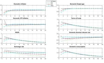
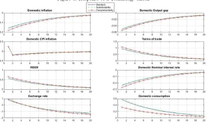
Figure 1: Response to a Domestic TFP shock
The responses of the output gap and domestic inflation are zero under the optimal policy rule.
Once we set domestic inflation and the output gap to zero, the policy rate will be lowered to follow
the path of the natural rate of interest. The exchange rate depreciates after the reduction of the
domestic policy rule, given that the foreign economy’s policy rate is constant in this case. This
both fixed at zero. The depreciation of the terms of trade will boost the growth of the actual rate
of output until it equals its natural level.
Consumption is lower in the open economy version than in the closed economy version. This
is attributed to the difference in the market clearing conditions between the two economies, give
that domestic output is not just absorbed by domestic consumption in the open economy, but by
foreign consumption as well. Also, under a technology shock, the economy will still suffer from
a decline in employment, similar to the closed-economy version of the model. Nevertheless, this
decline in employment is minimised in the open economy case also due to the offsetting effect of
the degree of openness of the economy.
The behaviour of the domestic inflation targeting rule closely resembles the behaviour of the
optimal policy. Despite having a nominal value less than the optimal policy rate, the domestic
inflation rule still has a contractionary policy stance as its real value (iH,t−πH,t+1) is above the
natural rate of interest. Also, the policy’s inability to guide inflation expectation to zero will lead
the terms of trade to depreciate by less than the required amount to close the output gap to zero.
The lack of depreciation in the terms of trade will lead to a negative output gap and negative
domestic inflation rates.
Under the exchange rate-peg regime, smoothing the terms of trade by keeping the exchange
rate fixed will result in higher volatility in the domestic variables. On the other hand, the main
difference between the CPI-targeting rule and the domestic inflation-targeting rule lies in the
behaviour of the terms of trade. The CPI-rule targets both domestic inflation and the terms of
trade. For this reason, the CPI-targeting rule will not allow the terms to depreciate enough to
boost output until it reaches its potential level, and this explains the hump-shaped in the terms of
trade and the exchange rate under the CPI-targeting rule. As a result, the output gap under the
CPI-targeting rule will be higher than the one under the domestic inflation-targeting rule.
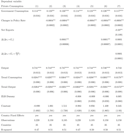
5.1.2 A Domestic Government Shock in the Open Economy:
The effect of a government consumption shock in the small open-economy follows the dynamics
of the same shock in the closed-economy version of this model: An increase in government
con-sumption will have a positive effect on the natural rate of output, and a positive response by the
effect of this shock is minimised by the degree of openness in the economy when compared with
the same shock in the closed-economy version of this model.
Given that domestic inflation and the output gap are set to zero under the optimal policy rate,
the increase in the natural rate of interest causes an appreciation in the nominal exchange rate.
This appreciation will sufficiently transmit to the terms of trade. The appreciation of the terms of
trade will, in return, dampen the growth of domestic output and keep it at an equivalent value to
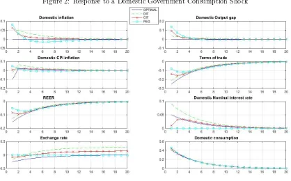
[image:28.595.89.507.255.515.2]its natural level.
Figure 2: Response to a Domestic Government Consumption Shock
The dynamics of the other policy rates follow their same behaviour under the technology shock,
but in an opposite manner. We notice that under a domestic inflation-targeting rule, the nominal
value of the policy rate increases above the neutral level of interest, but its real value is below
it, indicating an expansionary monetary policy stance. Moreover, this increasein interest rates
is not fully reflected on the exchange rate because of the inability of this policy rule to guide
expectations of inflation to zero levels. The less than required appreciation in the exchange rate
The overheating in domestic output will cause positive rates of domestic inflation, consequently.
Under the CPI-targeting rule, we also notice a hump-shaped response in the policy rate. This,
as explained above, is due to the fact that under this rule the terms of trade are also targeted by
the monetary authorities, in addition to domestic inflation. As a result, the policy rate starts to
increase until the point when the necessity of stabilising the terms of trade arises. While under
the exchange rate-peg regime, smoothing the terms of trade by allowing them to only appreciate
through domestic inflation causes more volatility in the output gap and domestic inflation.
Lastly, we notice that consumption in this open version of the model is at higher levels than
consumption in the closed version of the model under the same government consumption shock.
This is because the appreciation of the exchange rate boosts the purchasing power of domestic
households and in return, that increases domestic consumption of imported goods to the point
that domestic consumption exceeds domestic output. We observe the opposite under a technology
shock in the open economy, and this explains how the degree of openness minimises the crowding
out effect of fiscal policy on monetary policy.
5.2
Spillover Effect on the Domestic Economy
The structure of the model enables us to construct further analysis on the domestic small open
economy. In this regard, by modelling the foreign economy, we can capture the effect of shocks in
the foreign economy on domestic variables via the three important channels. The first is changes in
world demand for domestic goods, which is illustrated in the domestic market clearing condition.
The second is the price differential in the two economies which affects the competitiveness between
the two economies. The last, which is the vital one, is the interest rates differential between the
two economies. We only limit this analysis to one policy rule in the foreign economy, and that rule
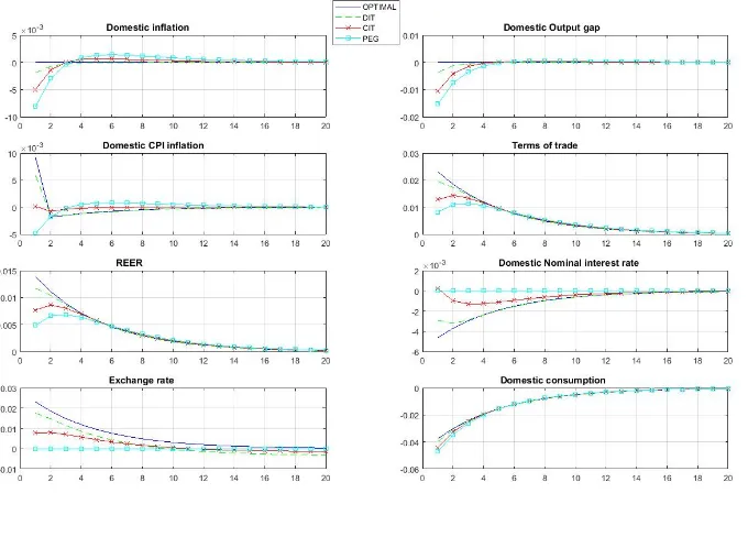
5.2.1 The Effect of a Technology Shock in the Foreign Economy on the Domestic Economy:
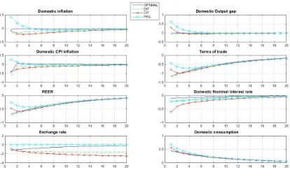
Figure 3: Response to a TFP Shock in the Foreign Economy
A shock in the foreign economy’s TFP causes growth in world demand for domestically produced
goods. The main channel in these dynamics is, as noted above, the interest rates differential
between the two economies. In this regard, given that the monetary authority in the foreign
economy will lower its policy rate to accommodate the expansion in the natural rate of output, the
domestic authorities should try to manage how its exchange rate should behave in order to achieve
internal stability in the domestic economy.
Under the optimal policy rule, the domestic policy rule aims to achieve a positive interest rate
differential against the foreign economy’s interest rate. This positive gap in the interest rates will
cause the terms of trade to appreciate to the extent that it keeps actual output at its natural
level. Thus, under the optimal policy rule, inflationary external demand for domestic products is
reduced by making domestic products more expensive for foreign households, and by increasing
Under the domestic inflation targeting rule however, the policy rate is lowered at a level
equiv-alent to the foreign economy’s policy rate. Nevertheless, its inability to manage expectation of
zero-domestic inflation expectations makes the terms of trade appreciate more than required,
caus-ing a negative output gap. The double dimensional structure of the CPI-targetcaus-ing rule will aim at
lowering the policy rate to close the negative gap of domestic inflation (its first target), and this
causes the actual output to grow above its natural level. Nevertheless, as the terms of trade start
reaching undesirable negative values, the policy rule is reversed to stabilise the terms of trade (its
second target).
Under the exchange rate-peg regime, the domestic authorities follow the rule conducted by the
foreign economy’s authorities. As a result, the domestic policy rule will be lower than the neutral
rate of interest. This expansionary stance will boost the actual rate of output to grow above its
natural level, causing inflationary pressure. Consistent with the analysis of shocks in the small
open economy, pegging the exchange rate causes smooth behaviour in the terms of trade, given
that they are only affected by the sticky prices of the two economies only. As a result, adopting
this rule will cause more volatility in the domestic variables (domestic inflation, the output gap).
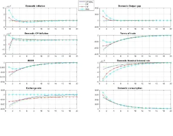
5.2.2 The Effect of a Government Shock in the Foreign Economy on the Domestic Economy:
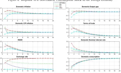
Under a government consumption shock in the foreign economy, the foreign economy’s policy rate
will increase to limit the inflationary pressure arising from the increase in demand. From the
uncovered interest rate parity condition, the relative increase in foreign interest rates will cause
downward pressure on the value of the domestic economy’s currency, and foreign demand for
domestic goods will also increase in this case. Thus, leaving the domestic policy rule unchanged in
this case will boost the actual rate of output to grow far beyond its natural level leading to high
levels of inflation.
Under the optimal policy rule, the gap between the interest rates is reduced to limit the
depre-ciation in the domestic currency. This depredepre-ciation will fully reflect on the terms of trade, leading
the actual rate of output to grow at a rate equivalent to its natural level, and this will cause zero
levels of domestic inflation. Limiting the depreciation of the domestic currency will also minimise
Figure 4: Response to a Government Consumption Shock in the Foreign Economy
We also notice that the domestic inflation-targeting rule fails, in this case as well, to guide
expectation of inflation to the zero-levels, despite the fact that the nominal value of the policy
rate, in this case, was above the value of the optimal policy rate. Under this rule, the gap between
the interest rates is minimised more than the optimal policy rule. Nevertheless, this interest rate
differential will not fully reflect in the exchange rate, due to the presence of non-zero domestic
inflation levels. The high level of depreciation in the domestic currency, in this case, will cause the
actual rate of domestic output to grow above its natural level leading to positive rates of inflation
in return.
Under the exchange rate-peg regime, the domestic authorities will follow the rate adopted by
the foreign economy’s monetary authorities in this case as well. This rate will cause the terms of
trade to only grow via the relative sticky prices in the two economies. The actual rate of output
will grow less than its potential level, causing a negative output gap and negative inflation rates as
a result. Thus, adopting the exchange rate-peg regime will lead the economy into recession because
of trade), in order to achieve internal stability (the output gap, domestic inflation). Under the
CPI-targeting rule, the policy rate is first increased to limit the high levels of domestic inflation
causing a less than needed depreciation in the terms of trade. However, the policy rule reverts
once domestic inflation starts going down. The terms of trade are never a concerning issue in this
case since the depreciation in the exchange rate is offset by the positive levels of domestic inflation.
This section highlights the main differences between the dynamics of this model and the one
used inGanelli 2003. In this model, the interest rates differential will affect the purchasing power
of the domestic consumers, due to the reaction of monetary policy to changes in aggregate
de-mand. This will result in a contradictory effect between domestic government consumption and
foreign government consumption on domestic private consumption, both in the complementarity
and substitutability case.
5.3
The Substitutability Case
In this section we illustrate how the dynamics of the model change, once we incorporate government
consumption as a substitute to private consumption10:
5.3.1 A Technology Shock in the Open Economy:
The response of the natural rate of interest to a technology shock, in this case, is consistent with
its response under the other cases. The natural rate of interest is reduced in this case as well
to accommodate the expansion in the natural rate of output. Nevertheless, the reduction of the
natural rate of interest, in this case, will be less than all of the other cases. This is attributed
to the fact that output is more sensitive to changes in interest rates under the substitutability
assumption, as noted earlier. Also, the positive effect of a technology shock on the natural rate of
output is higher than all of the other cases.
Similar to all the other cases, under the exchange rate-peg rule and the CPI-targeting rule, the
relative smoothing of the terms of trade will cause more volatility in domestic inflation and the
output gap.
5.3.2 A Government Shock in the Open Economy:
Government consumption will have an adverse effect on output in this case. The role of monetary
p