Polarization and the Middle Class in
China: a Non-Parametric Evaluation
Using CHNS and CHIP Data
Khan, Haider Ali and Schettino, Francesco and Gabriele,
Alberto
UNIVERSITY OF DENVER, COLORADO, US, UNIVERSITY OF
CAMPANIA L.VANVITELLI, NAPLES, ITALY
December 2017
Online at
https://mpra.ub.uni-muenchen.de/86133/
Polarization and the Middle Class in China: a Non-Parametric
Evaluation Using CHNS and CHIP Data
Haider Ali Khan, JKSIS, University of Denver (Colorado, USA) –[email protected]
Francesco Schettino, University of Campania “L. Vanvitelli” (Naples, Italy) –
1. Introduction
By the time of its founding in 1949, PRC was one of the poorest countries in the world. The revolutionary Chinese government and people carried out a fundamental socio-economic transformation and embarked on a path of moderately dynamic economic growth. This first, initial stage of PRC’s socioeconomic development lasted about three decades, spanning the 1950s, 1960s and 1970s. Since the late 1970s, China has launched a series of progressively deeper market-oriented reforms, without relinquishing the dominant role of the State and of the Communist Party in key areas of the economy. The cumulative result of these major, albeit gradual, changes has been the transition of China’s formerly centrally-planned socialist fabric to a new and unique socioeconomic system. This new system has proven so far to be endowed with a relatively high degree of stability, consistency and sustainability, in spite of the extraordinary speed of its incessant internal evolution. In the remainder of this paper, we will refer to the post-1978 and pre-1978 periods of PRC’s economic history as the reform and pre-reform period, respectively.
By the end of WWII, China’s per capita GDP was only slightly over 20% of the world average and 5% of that of the US. On balance, China’s overall growth performance was no better than that of India and of most other backward countries. It looks particularly gloomy when compared to the then-unprecedented success of two of its capitalist neighbors and rivals, Japan and South Korea. Both of them, starting from different levels of economic development and enjoying – quite differently, to be sure, from internationally isolated PRC – preferential access to the US market, investment and technology flows had managed to substantially reduce the development gap separating them from the leading economic superpowers.
Conversely, since the inception of the market-socialist reforms in the late 1970s, China’s growth skyrocketed. Per capita GDP increased eightfold over the period, from about 1000 to 8000 USD (1990). By some standards, it can be argued that China’s catching up process, since the inception of the reform period, has outpaced those of Japan and South Korea in the preceding one, setting a new world record. During the first half of the 2010s, China’s economic growth progressively slowed down, recording a rate of about 7% per year– still an extremely high figure by world standards. This is still more remarkable when we take into account, inter alia, the marked slowdown in international trade caused by the persistence of what has been dubbed “Secular Stagnation” (see Summers, 2014) in major leading economies.
It is well known that the impressive reduction of poverty in the last few decades was accompanied by a clear increase in economic disparities. The very significant gains in inequality reduction achieved in post-revolutionary China during its first phase of development (the Gini coefficient declined from 0.558 in 1953 to 0.317 in 1978, UNDP, 2016) were subsequently erased to a large extent. Indeed, while the impressive GDP growth almost completely eliminated absolute poverty, the change in the shape of distribution was equally strong, generating a new class composed by very rich people, an event that, to some extent, falls into contradiction with the concept of a socialist-oriented country.
“hollowing out” of the middle class (see, among others, Esteban and Ray, 1994, 1999, 2011; Duclos et al., 2004; Esteban et al., 2007). Especially in a period of “secular stagnation,” the role of the Chinese middle class is indeed crucial, not only for the local economy but for the world as a whole because it is now one of the main components of the global effective demand.
In this paper we focus on polarization by using the methodology of using an analytical approach to Relative Distribution Tools.In order to focus on the polarization features in the last 2 decades, an overview of the principal contributions on the conceptualization of middle class and polarization (in general and for PRC) is presented in Section 2. Section 3 describes the data sets. Section 4 presents the statistical tools and discusses the results. Section 5 presents conclusions including possible political economic implications of our statistical results.
2. Middle class and Polarization
2.1 A conceptual overview
Since the turn of this century, polarization has come to the forefront of international socioeconomic research, due to its paramount role in the analysis of the evolution of income, consumption expenditures and wealth1 distribution. Polarization methodology---particularly in our relative distribution version--- can be used to examine the potential for social conflicts, economic growth and development as well.2 The logic of this method is that polarization is one fruitful attempt among others3 at measuring the objective segregation among social groups with respect to their respective material well-being, which is in turn identified with the degree of within-group similarity and between-group disparity. The concept of polarization is thus intrinsically related to that of socio-economic classes and class-consciousness – although not exclusively with the Marxian or Weberian concepts (other ones are that of middle class and of marginal/excluded class). Polarization describes the degree to which a population is segregated into groups in a society (Gradín, 2000: 457). It detects the presence or disappearance of such groups in a distribution (Chakravarty, 2009), indicates how individuals and groups feel toward one another (Duclos, Esteban and Ray, 2004), and captures the phenomena of a diminishing middle class or a divided society (Zhang and Kanbur, 2001).
According to Esteban and Ray (1994: 824), the concept of polarization has three features: a small number of groups, a high degree of homogeneity within each group (the so-called identification ingredient), and significant heterogeneity between groups (the so-called alienation ingredient). It is a powerful indicator, of the objective social conditions that can be expected to bring about subjective (psychological, sociological and ultimately political) within-group identification and between-group alienation on the part of individuals belonging to different social groups - more so than measures of income or wealth inequality and poverty. Thus, it can be seen as a warning red
1
In the remainder of this paperwe will use simply the term “income distribution,” implicitly referring both to monetary (income and expenditures) and not-monetary distribution studies.
2
See among others Esteban and Ray, 2008, Esteban and Schneider, 2008 (and more generally, the Journal of Peace Research, Vol. 45, No. 2, Special Issue on Polarization and Conflict, March 2008); recently, Gochoco-Bautista et al., 2013; Corral et al., 2015.
3
flag urging corrective interventions, and ultimately (unless such policy actions are promptly and effectively carried out) as a predictor of future social conflict.
The concept of polarization is intuitively associated with the structural features of middle class: as a first approximation, polarization implies a hollowing out of the middle class and a fattening of one or both tails of the distributional curve. Actually, the terms middle class and polarization are, by themselves, etymologically quite clear and intuitive. Limiting our focus on “objective” income distribution analysis,4 it is apparent that (barring the extreme case of perfect equality) in every (national) society5 some people are rich, some are poor, and some are not-so-rich and not-so-poor. Utilizing heuristically and neutrally the term “class” to refer to each of these groupings, the last one can naturally be termed “middle class” – i.e., the middle class is simply that part of the population that, in terms of income (or consumption expenditures), is in the middle between the “rich” and the “poor.”6
From the viewpoint of the history of socioeconomic thought, the modern concept of class came to the fore along with the analysis of the capitalist system. The main schools of thought that accorded a paramount role to class are the Marxian and the Weberian ones. For Marx, class is a central abstract category aimed to understanding the internal laws of the motions of capitalism. The two core classes are bourgeoisie and proletariat, identified according to their opposite position vis-a-vis the ownership of capital. Yet, a third, less clearly defined intermediate class (the middle class) also exists, mainly composed by professionals and petty traders. Classes are “real social processes reflected in thought which help to reveal the essential class dynamics of the capitalist mode of production” (Lekhi, 2001, p.161). It is therefore at this relatively high level of theoretical abstraction that Marx and Engels put forward their well-known belief in the tendency towards the polarization of capitalist society in two opposite classes in the Manifesto: “Society as a whole is more and more splitting up into two great hostile camps, into two great classes directly facing each other: bourgeoisie and proletariat (Marx and Engels, 1848))” and, more precisely in Das Kapital, discussing the general law of the accumulation of capital (Book I, Ch.23). Weber analyzes class in a more general context of social stratification, where class is one dimension of social structure along with another, social status. He also attaches great relevance to the concepts of power, domination, and communal and societal action (see also Coser, 1977; Lekhi, 2001; Shortel, 2016). In spite of their differences, Marx’ and Weber’s concepts of class are to some extent similar in two important
4Many sociological and psychological studies have explored the relevance and diffusion of the “middle class values”
and the varying subjective degrees of identification with the middle class on the part of different social groups that might be very distant from the latters’ objective belonging to a given income or wealth. For instance, it is well-known that most Americans tend to identify themselves as middle class, more so than their European counterparts. This difference is partly related to moral and ethical values attached to the term in different cultural contexts, and to the
intrinsically different meaning that the terms “middle class” and “working class” have evolved into in different
countries (see also Sosnaud et al., 2013; Hout, 2008; Jackman and Jackman, 1983).
5
Other studies adopt an international, or even a worldwide approach, utilizing concepts such as between-country inequality and, in some cases, global polarization and global middle class. The global middle class is usually identified with the worldwide aggregation of uneven population groups belonging to the population of many developed and developing countries, all of them unified by the characteristic of being endowed with a sufficient high purchasing power to be able to buy a certain bundle of modern tradable goods and services. The global middle class is composed by households with an income equal to or higher than a minimum threshold (set in international dollars). Given the focus of the analysis, many studies do not even establish any upper bound to the global middle class, thereby implicitly identifying the middle with the upper global class and thus classifying substantially the world population in only two classes: those who can accede to a minimum bundle of modern tradable consumerist items and those who can’t. See AfDB, 2011; OECD, 2011; Corral et al., 2015.
6Perceptive and rigorous scholars like Murakami (1997) have used the term “middle masses” which avoids the Marxist
respects: they see the economic dimension of class as key, and define a particular class location according to its links with other classes.7
In the domain of statistics the concept of class is straightforward and uncontroversial although not identical with the above conceptualization. A class is a grouping of values by which data is binned for computation of a frequency distribution (Kenney and Keeping 1962, p. 14). Thus, in the case of income distributions, an income class is composed by households in which income falls between the limits of a range of values (called a class interval). Here the terms class and grouping are interchangeable and unconnected with any substantive social, political or economic theory. Therefore, when the term middle class is used neutrally (i.e., independently from any conceptual elaboration of its socioeconomic function) the middle class is simply identified with “middle -income households” – i.e., households with an income that falls in an arbitrarily determined interval centered around the median (see Alichi et al., 2016).8 Of course, this use of the term class in the context of income/ wealth distribution does not imply (or deny) that middle-income households – or, by the same token, low or rich-income households – form a class in the above-mentioned, strong sociological sense. We might call this meaning of class, which is in fact purely quantitative, neutral and unambiguous, a “weak” meaning. In the domain of applied research – as opposed to that of purely theoretical thinking – it is only after reaching robust quantitative results that analysts can (if they deem it meaningful) put forward an interpretation pivoting on the “strong,” socioeconomic concept of class.
Middle class (the boundaries of which are set according to subjective9 criteria by researchers themselves) and polarization are mostly analyzed both in a cross-country and a historical perspective. They aim to find out whether the middle class has been evolving over time to constitute a larger or smaller share of the population, and/or capturing a larger or smaller share of total national income.10 In this context, polarization can be understood as a tendency on the part of the population and/or of national income to concentrate itself around two opposite “poles” (the rich and the poor).
Thus, both terms naturally point towards an analytic and descriptive distributional vision of society that is rather clear-cut, essentially constituted by just three major groupings. If the third, intermediate group tends to wither out while the population concentrates itself towards the upper or the lower tail, a polarization process is going on. This “pure” form of polarization can be estimated with two relatively straightforward and unambiguous methodologies. One consists in choosing arbitrarily a statistical interval setting the boundaries of the middle class (for instance, defining it as consisting of households with 50-150 percent of median income), and using it to estimate the
7
After Marx and Weber, the idea of class has remained a central one in the domains of sociology and (to a lesser extent) of economic science, and has been subsequently discussed by many analysts, scholars, and politicians. This debate has focused mainly on conceptual and theoretical issues, such as the identification of social classes, their
functional mutual interactions, and the relationship between objective belonging to one or another class grouping and its subjective perception.
8Alichi et al., define “middle
-income households” as those with an income falling in an interval ranging from 50 to 150 percent of median income, and show that their weight in total US population fell from 58% in 1970 to 47 % in 2014 (Fig 3, p. 5).
9
Subjective is not synonymous of haphazard. Researchers can legitimately adopt various and possibly diverging criteria in setting the boundaries of the middle class, according to their different ex-ante theoretical views and analytical goals.
10
relative share on middle class households in the total population. The other is based on the Wolfson index (W), which estimates the relative size of the middle class measuring the degree of clustering around the median (see also Foster and Wolfson , 1992 and Wolfson, 1994, Alichi et al., 2016).
Since the turn of the century, both the concepts and measurements of the middle class and polarization have been the object of novel theoretical and statistical elaborations. In different analytical contexts these theoretical efforts have ended up referring to concepts that are quite different from the original ones. The most important one is that of multi-polar polarization. The modern concept of polarization was pioneered by Esteban and Ray, 1994. This approach is reasonable, as it allows to extend the concept of polarization to cover a much wider set of possible states of the world. If the number of groups is greater than three, the result is multi-polar polarization. In the recent literature on the statistical measurement of polarization, multi-polar polarization refers to the “clustering around local means of the distribution, wherever these local means are located on the income scale” (Chakravarty, 2015, p. vii).
2.2 Middle class and Polarization in PRC
Since the inception of the industrial revolution, notwithstanding the numerous historical examples of successful catching up processes in many backward countries, a long-term trend towards ever-increasing polarization has prevailed worldwide. However, since the last decades of the XXth century this trend appears to have been reversed, thanks mostly to the exceptional growth performance of the PRC (and, to a lesser extent, of India). Yet, inside PRC itself, it has been accompanied by a trend towards increasing within-country inequality . More recently, following the increasing attention by the international research community, crucial social and political implications are being grasped. As a result, analysts have begun to carry out studies that focus specifically on polarization. These contributions aim, first of all, to determine whether or not mounting inequality implies also a trend towards increasing polarization, and (if this is in fact the case) to analyze in depth what kind of polarization – mainly, bi-polar or multi-polar – is taking place, particularly in China.
The earliest studies showed a marked degree of geography-related polarization between urban and rural areas and between coastal and inland provinces (see Kanbur and Zhang, 2001). Polarization also appeared to be on the rise, albeit moderately, although countervailing trends also emerged. During the early reform period, the rural-urban gap diminished, thanks to the success of initial agricultural reforms and the boom of TVEs. Yet, the latter also caused increasing polarization between more and less advanced rural communities. More recently, in the 1990s, polarization appeared to be stable, but afterwards an unambiguous rising trend became apparent. Urban polarization, in particular, has been driven by the liberalization of the labor market that has led to a widening of wage dispersion and – to some extent – unemployment, by the decrease in subsidies and by the emergence of new sources of income, such as self-employment, profits, and financial rents (see Bonnefond and Clément, 2012; Wan and Yang 2014).
income. Urban polarization is caused mainly by declining subsidies, the liberalization of labor markets and the reforms of state enterprises. Bonnefond and Clement (2012) conclude that polarization in China is a by-product of the efficiency-first development strategy implemented since the beginning of the reform period. They also note that the Chinese government has been increasingly aware of the gravity of this problem, leading to the adoption of the concept of “harmonious society” and to the inclusion of significant inequality and polarization reduction goals in the 11th and 12th five-year plans.
Wan and Wang (2015) analyze polarization in China on the basis of data from the China Statistical Yearbooks and the China Household Income Project (CHIP), and use the decomposition technique in order to attribute the change in polarization into a growth and a redistribution component (Shorrocks, 1982). Since the mid-1980s to the mid-1990s,11 nationwide polarization increased from a low initial base due to rising alienation, while identification was declining. However, this trend was not homogenous. In rural areas, polarization surged until the early 1990s and remained stable afterwards. In urban areas the peak was in 2003, followed by a slight decline until the end of the decade. The authors also present a more detailed analysis carried out for the 2002-2007 period, identifying migrants as a distinct subgroup of the population. In this period, overall polarization in China was driven mainly by the increasing alienation between rural citizens. Migrants were improving their lot more than those who remained in the countryside and – in spite of the persistence of hukou-based discrimination in the cities – were becoming more homogeneous with urban citizens. The dominant polarizing income source has been investment income, especially so in a context where the labor share in national income was rapidly falling. Investment income has been “driving polarization and segregation between investors and laborers… investors are … in the rich segment of a society and benefit more as financial markets develop… making the country more polarized” (Wan and Wang (2015) p. 13). On the basis of their findings, Wang and Wan recommend to reform the hukou system in order to equalize the conditions of all urban workers, and to strongly promote agribusiness and further rural industrialization.
Piketty et al (2017), in a study focusing on capital accumulation, private property and rising inequality12 in China, also identified a long-term trend towards polarization in the 1978-2015 period. Their results (obtained with a methodology that combines survey, fiscal and national account data, and which are therefore only roughly comparable to those presented in this paper) show that “the share of national income going to the top 10% of the population has increased from 27% in 1978 to 41% by 2015, while the share going to the bottom 50% has dropped from 27% to 15%. In other words, top 10% income earners in China used to earn 5 times more than bottom 50% earners, and they now earn 13.5 times more. Over the same period, the share going to the middle 40% has been roughly stable (around 45% of total income) (Piketty et al (2017)p.31).
3. Data description
The NBS (National Bureau of Statistics), PRC’s official statistical agency, produces and publishes a vast array of information, which is presented at various levels of aggregation. However, since the early 1990s, many studies on China’s income and wealth distribution have opted for using other
11
The authors were not able to estimate polarization trends in some periods due to the lack of available data.
12
statistical sources, preferring Household Surveys collected by organizations different from the NBS, due mainly to two reasons. First, independent researchers cannot access NBS microdata. Second, non-NBS household surveys typically collect a larger number of potentially useful variables. There are seven non-NBS household surveys relevant for distributional analysis:
i) CHIP – China Household Income Project;
ii) RUMiC – Rural-Urban Migration in Indonesia and China; iii) CHNS – China Health and Nutrition Survey;
iv) CGSS – China General Social Survey; v) CFPS – China Family Panel Studies;
vi) CHARLS - China Health and Retirement Longitudinal Study; vii) CHFS - China Household Finance Survey.
These surveys differ from one another in scope and design and cover various periods and sets of variables. Some of them are richer or more representative than others (for an exhaustive discussion of each survey’s pros and cons see Gustafson et al., 2014). However, the main criterion of choice depends chiefly on researchers’ analytical goals. As the main objective of this paper is to develop an estimation of PRC “well-being” distributional features, taking into account both monetary and non-monetary variables, we – along with several other researchers – opted for using, in a mutually complementary fashion, data produced by both the CHIP and CHNS surveys, on the basis of three considerations. First, CHIP data jointly cover a longer time-span (1980-2013) than other surveys. Second, its structural design has been consistently maintained by the NBS researchers in many stages of the data generating process, covering many provinces. Third, CHIP 2002 has been included in the LIS Cross National Data Centre (Luxembourg) on November, 2012. However, CHIP data mainly consist of monetary (income) variables, while little information is provided on wealth and non-monetary ones. Conversely, the CHNS HH Survey – while less detailed with respect to income information proper – provides rich information on health and nutrition variables. Moreover, it has been carried out on the basis of a larger number of subsequent rounds (almost 10 from 1989 to 2011; see Ward, 2014). Yet, CHNS’s coverage of province level units is smaller than CHIP’s, and it does not include any of the four municipalities.
The China Health and Nutrition Surveys (CHNS) were conducted by the Carolina Population Center, University of North Carolina for a longer time span: 1989, 1991, 1993, 1997, 2000, 2004, 2006, 2009 and 2011. The data, in panel form, were collected on about 4,400 households (19,000 individuals) in nine provinces in China: Guangxi, Guizhou, Heilongjiang (from 1997), Henan, Hubei, Hunan, Jiangsu, Liaoning, and Shandong. This selection was mainly driven by the high degree of diversification of these provinces from an economic, demographic and, more broadly, a social point of view. The provincial capital and a lower income city were selected (when this choice was feasible according to the availability of data), while the villages and townships within counties, and urban and suburban neighborhoods within cities were selected randomly (see also Liu 2008).
4. Polarization profiles
4.1 The Relative distribution method
The Relative Distribution approach is a non-parametric one that combines the strengths of summary polarization indices with the details of distributional change offered by the Kernel density estimates (see Handcock and Morris, 1998, 1999, Alderson et al., 2005, Massari, 2009, Borraz et al., 2011, and Alderson and Doran 2011, 2013, Clementi and Schettino, 2015, Clementi et al., 2015, Clementi et al., 2016). This technique assesses the evolution of the middle class and the degree of household income polarization in different low, middle and high-income countries.
In order to employ the relative distribution method13, it is necessary to single out one of the two populations (same variable, in two different years), refer to it as the “comparison” population, and refer to the other as the “reference” population. More formally, let Y0be the income variable for the reference population and Y the income variable for the comparison population. The relative distribution of Y to Y0is defined as the distribution of the random variable:
0 ,
R F Y (1)
which is obtained from Y by transforming it by the cumulative distribution function of Y0, F0.
While this transformation is not widely used or understood in the social sciences, it is a very useful one, because R measures the relative rank of Y compared to Y0. It is continuous on the outcome space [0, 1], and we will call r, a realization of R, the relative data. The relative data can be interpreted as the set of positions that the income observations of the comparison population would have if they were located in the income distribution of the reference population. The probability density function of R, which is called the “relative density,” can be obtained from the ratio of the density of the comparison population to the density of the reference population, evaluated at the relative data r:
01
1
0 0 0
, 0 1, 0,
r
r r
f F r f y
g r r y
f y f F r
(2)
where f
and f0
denote the density functions of Y and Y0, respectively, and 1
0 ry F r is the quantile function of Y0. The relative density has a simple interpretation, as it describes where households at various quantiles in the comparison distribution are concentrated in terms of the quantiles of the reference distribution. As for any density function, it integrates to 1 over the unit interval, and the area under the curve between two values r1 and r2 is the proportion of the
comparison population whose income values lie between the th 1
r and th 2
r quantiles of the reference
population.
This method provides intuitive tools that can be used formally to distinguish between growth, stability, or decline at specific points of the income distribution(s). In fact, the case in which the relative density function shows values equal to 1, it simply represents that the two populations have
equal density at the th
r quantile of the reference population. A value greater than 1 implies that the comparison population has more density than the reference population at the th
r quantile of the latter. Finally, a function value inferior than 1 indicates the comparison population has less density in the considered quantile.
Therefore, one of this method’s major advantages consists in the possibility to decompose the relative distribution into changes in location and in shape. In other words, it allows to separate the
13
measures usually associated with changes in the median (or mean) of the income distribution by the “pure” distributional features change (including differences in variance, asymmetry and/or other distributional characteristics) that could be easily linked with several other factors, for instance, polarization. Formally, the decomposition can be written as:
0
0 0 0
Overall relative Density ratio for Density ratio for density the location effect the shape effect
,
r L r r
r r L r
f y f y f y
g r
f y f y f y
1 2 3 14 2 43 14 2 43
(3)
where f0L
yr f0
yr
is a density function adjusted by an additive shift with the same shape as the reference distribution but with the median of the comparison one. The value is thedifference between the medians of the comparison and reference distributions. Indeed if the two distributions have a different median, the “location effect” is increasing in if the comparison median is higher than the reference one. The opposite happens if the “location effect” is decreasing. The “shape effect,” represents the relative density net of the location effect and it isolates redistributive movements occurring between the reference and comparison populations. For instance, we could observe a shape effect function with U-shaped pattern if the comparison distribution is relatively more spread around the median than the location-adjusted one. Thus, it is possible to determine whether there is polarization of the income distribution (increases in both tails), “downgrading” (increases in the lower tail), “upgrading” (increases in the upper tail) or convergence of incomes towards the median (decreases in both tails).
The relative distribution approach also includes a median relative polarization index (MRP), which is based on changes in the shape of the income distribution to account for polarization. This index is normalized so that it varies between -1 and 1, with 0 representing no change in the income distribution relative to the reference year. Positive values represent more polarization and negative values represent less polarization – i.e., convergence towards the center of the distribution. The MRP index for the comparison population can be estimated as (Morris et al., 1994, p. 217):
1 4 1 MRP 1, 2 n i i r n
(4)where ri is the proportion of the median-adjusted reference incomes that are less than the
h t
i income from the comparison sample, for i 1, ,n, and n is the sample size of the comparison population.
The MRP index can be additively decomposed into the contributions to overall polarization made by the lower and upper halves of the median-adjusted relative distribution, enabling one to distinguish downgrading from upgrading. In terms of data, the lower relative polarization index (LRP) and the upper relative polarization index (URP) can be calculated as follows:
/ 2 1 8 1 LRP 1, 2 n i i r n
(5)/ 2 1
8 1 URP 1, 2 n i i n r n
with MRP 1
LRP URP
2 . The MRP, LRP and URP range from -1 to 1, and equal 0 when there
is no change.
4.2 Main results14
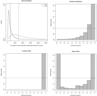
[image:13.595.57.542.355.617.2]In this Subsection we present the principal results of the polarization analysis using CHNS and CHIP datasets. For the CHNS, we estimated the evolution of the variable per capita HH income using the price index for 2011.15 For CHIP, we used the variable Total household income per capita.16 Following the methodology proposed by Song et al., (2008), we weighted17 the CHIP samples by wave, expressing all data in 2012 prices and taking into account regional variability.18 The traditional measures of income polarization---e.g., Foster and Wolfson (1992) and Duclos et al., (2004),19 ---substantially confirm the last decade’s worsening trend of income distribution (Wang and Wan, 2015). It seems that, similar to the case of inequality indices, the peak has been reached in the mid-2000s decade, and in last years a reduction, albeit slight, is detectable. Urban households generally present a higher degree of polarization as compared with the rural ones (Table 2).
Table 1 – Polarization Measures by Wave and Survey
CHNS CHIP
All Urban Rural All Urban Rural
FW DER FW DER FW DER FW DER FW DER FW DER
1989 0.337 0.228 0.229 0.196 0.406 0.243
1991 0.335 0.225 0.237 0.194 0.373 0.236
1993 0.393 0.241 0.322 0.223 0.419 0.247
1997 0.367 0.234 0.300 0.219 0.404 0.240
1999 0.401 0.262 0.280 0.214 0.286 0.216
2000 0.403 0.252 0.335 0.235 0.431 0.243 0.393 0.258 0.283 0.213 0.294 0.220
2001 0.408 0.264 0.286 0.215 0.294 0.219
2002 0.451 0.269 0.285 0.214 0.307 0.224
2004 0.470 0.267 0.429 0.250 0.472 0.236
2006 0.500 0.284 0.423 0.263 0.513 0.247
2009 0.463 0.270 0.398 0.256 0.464 0.240
2011 0.432 0.259 0.351 0.236 0.469 0.269 0.398 0.249 0.305 0.217 0.338 0.234
2012 0.388 0.249 0.306 0.219 0.332 0.234
2013 0.383 0.256 0.290 0.222 0.325 0.237
14
For sake of brevity the results of covariates analysis has been include in Appendix 1.
15
The selected variable label is hhincpc_cpi,extracted from “Master_Constructed_Income_201410\hhinc_pub_00.dta” file.
16The variable was obtained dividing “
Total income” (P201) by “Member number within household” (P102), variables
contained in the file “DS0001[Urban Individual Income, Consumption, and Employment]\21741-0001-Data.dta”.
Analogous calculations have been conducted to estimate the total income per capita of rural and migrant households.
17
The population features data taken from NBS dataset.
18
The deflator source is the NBS dataset.
19
Figure 2 – Relative polarization indices by year – CHNS data (2011 as Comparison Distribution)
Figure 3 – Shape effect by year – CHNS Data – (1989 as Reference Distribution)
Figure 2 quantifies this tendency taking into account as comparative distribution the 2011’s one, and moving from 1989 to 2009, the reference’s distributions. The polarization trend is also confirmed in the period as a whole. It is important to note that the decreasing trend of MRP-LRP-URP is due to the fact that the more the reference year is close to the comparison one, the lower is the polarization degree.20 Overall,for each reference year the analysis confirmsthe fact that the MRP is principally driven by the LRP. In other words, in the considered period the Chinese middle class has moved mainly to the lowest deciles of the distribution. However, this “pure distributional” effect has been largely mitigated by the impressive GDP growth. Figure 3 presents the Shape effect change in the period, as a whole. In Figure 5, 1989’s distribution has been taken as the reference one while the comparison ones move from 1991 to 2011. From another point of view, it shows the hollowing out movement of the middle class; at the same time, a significant tendency towards polarization on the top and bottom deciles of the distribution is here confirmed.
The same exercise was performed on CHIP data, for the waves (2002-2013). As expected, the results are quite similar, and substantially confirm the trends revealed by the analysis of CHNS data (Figure 4). Summarizing, we can say that the crucial role of the impressive GDP growth of last decade (left-bottom graph – location effect) hides the significant “pure” distributive change (right -bottom graph – shape effect) that has gone in the direction of an increasing polarization, driven principally from the bottom deciles of the distribution (MRP=0.744; LRP=0.831; URP=0.656). Thus, analyzing the results as a whole, we can affirm that many households who used to belong to the middle income classes experienced no or relatively modest income increases. Therefore, their relative position worsened, and they moved from the central to the lowest decile of the distribution. This overall distributional outcome has been the product of many complex, overlapping and mutually interrelated factors. Among the most relevant the following are probably the most noteworthy. Changes in labor markets led to a widening of income differentials and to the emergence of new categories of urban workers, such as the self-employed and those hired by private firms (the relative positions of which worsened with respect to SOE and public employees) and migrants (who were penalized by their lack of hukou registration status, but improved their lot with respect to many other rural residents). Many private entrepreneurs became rich, some of them very rich. The fast but uneven expansion of access to basic amenities (i.e., water plant and flush-in house facilities) and to not-so-basic, human capital-enhancing services such as higher education also played a role21
20
Relevant distributional changes occur normally in a medium/long period.
21
Figure 4 –Relative distribution results - CHIP data 2002-2013
5. Concluding Remarks
Since China launched a series of progressively deeper market-oriented reforms from 1978-9 onwards, growth has accelerated but inequality has also increased. The new and unique Chinese socioeconomic system is still in transition but relatively stable. It can be argued that China’s catching up process since the inception of the reform period has outpaced those of Japan and South Korea earlier, setting a new world record.
A historical comparison shows that the rapid decline in inequality that occurred in post-revolutionary China during its first phase of development has been reversed during the market-oriented reforms period. Crucially, this has also led to rapid polarization in the 21st century in particular. While the topic of general “inequality” in China has been studied relatively intensely, less attention has been paid to the polarization phenomenon. Polarization, as opposed to inequality, has the characteristic of showing scientifically distinct distributional problems as features related to the formation, consolidation or the hollowing out of the middle class.
movements of the majority of the population towards higher levels of income (those that only belonged to the highest deciles at the beginning of the period).
The most important feature of the method we employ consists in the possibility of separating the overall effect in the location (growth) and shape (“pure distribution”) of the statistical distributions. Following this methodological step, we obtain some new results that provide a novel interpretation of the Chinese distributional inequalities in terms of the relative polarization indexes. The location effect shows that a large part of the overall effect is due to the distribution’s (median) right-shift, a clear consequence of the huge GDP growth of last decade(s). When excluding this growth-location effect, a typical polarization profile emerges. This is nothing other than the so-called shape effect. More specifically, the typical hollowing out of the central deciles of the distribution in PRC has been indeed accompanied by “fattening” of both tails of income distribution.
These results seem to be in opposition to the widely shared received idea that in the last decades the Chinese middle class consolidated its status, increasing both in terms of per capita income and in number. In fact, if we look merely at the “pure distributional” effect, our analysis tells that during the reform period, the Chinese middle class has moved mainly to the lower deciles of the distribution. However, this apparent contradiction can be statistically and economically solved by adding the other component of the overall effect, i.e. the location one.
Thus, the method we employed enabled us to examine critically the idea that the impressive GDP growth of last decade created a growing the Chinese middle class that will continue to grow. Our results show that scientifically there is no firm ground for basing such optimism regarding the growth of a middle class in PRC since many members of this class are being driven now to the bottom deciles of the distribution. As a consequence, as growth slows, unless countervailing policies are undertaken, polarization will reveal itself more sharply, and might eventually lead to increasing distributional and related political conflicts in PRC.2223
22
These results are consistent with the analysis of results of Khan(2017) and Khan(2010) that use different methodologies.
23
The risk of increasing social unrest has been clearly identified by PRC leaders and many other observers. According to Prof. Deng Chundong, dean of the Academy of Marxism of the CASS (Chinese Academy of Social Sciences), “since reforms and opening up, the gap between rich and poor, regions and industries has been expanding. China is in a crucial
period of reform, but also in a period of highlighted contradictions….there is a high incidence of social contradictions,
which are often acute, and even occur as group incidents. How to realize social stability and promote social harmony
Appendix 1
–
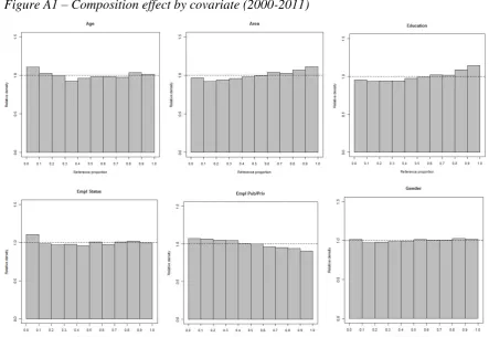
Covariates analysis
The main aim of this Subsection consists in pointing out the principle covariates considered as drivers of the (relative) polarization, in the sense of Handcock and Morris (1998, 1999). Wan and Wang (2015) deeply inquire on the polarization changes by decomposing income sources. Differently, and to some extent, in order to provide a more exhaustive analysis, we decompose the detected polarization by household features, applying the covariate adjustment technique (Handcock and Morris, 1998, 1999) as modified by Clementi and Schettino (2015).
[image:20.595.58.544.357.747.2]Since the covariates selection, according to the literature, is commonly linked to households’ assets and/or household-head characteristics, we employ this methodology on CHNS data that, as sketched out in previous sections, is richer than CHIP in terms of information we need. The selected variables for our analysis are connected to household location (Area and Stratum); HH head’s age, its gender, HH head’s education, its occupational status and the sector of employment are evaluated as proxies for socio-demographic features. Moreover, two variables (Source of drinking water and Typology of Toilette in the dwelling), representative of HH’s assets, have been taken in consideration. In Table 2, descriptive statistics are reported.
Table A1 – Descriptive statistics by covariate
Mean Income Population Share Gini
2000 2011 2000 2011 2000 2011
Age
less than 40 5,493 17,546 24.71 10.54 0.45 0.45 41-60 5,824 16,858 51.19 52.10 0.43 0.46 61-80 5,305 14,328 22.55 34.19 0.50 0.45 more than 80 4,337 16,272 1.56 3.17 0.49 0.47
Area
Urban 7,393 19,177 32.96 42.89 0.43 0.42 Rural 4,721 13,695 67.04 57.11 0.45 0.47
Stratum
Urban Neighborhood 7,995 21,022 15.70 27.63 0.40 0.38 Suburban Village 6,846 15,836 17.26 15.26 0.45 0.49 County Town Neighborhood 5,875 16,461 16.35 17.66 0.42 0.45 Rural Village 4,349 12,457 50.69 39.44 0.45 0.48
Nationality
Han 5,772 16,302 87.43 90.78 0.45 0.46 not Han 4,420 13,532 12.57 9.22 0.45 0.46
Gender
Male 5,481 15,926 86.16 79.41 0.45 0.46 Female 6,352 16,513 13.84 20.59 0.46 0.45
Level of Education
Less than technical degree 5,161 13,762 88.94 80.60 0.45 0.46 At least Technical Degree 9,144 25,539 11.06 19.40 0.40 0.36
Presently Working
No 5,511 14,308 26.24 41.10 0.48 0.45 Yes 5,634 17,260 73.76 58.90 0.44 0.46
Type of Work Unit
Public 8,357 24,676 21.90 14.86 0.37 0.37 Private 4,829 14,541 78.10 85.14 0.46 0.46
Major Source of Drinking Water ground water 4,632 12,876 38.45 27.37 0.45 0.48 open well 3,953 15,865 6.45 1.61 0.51 0.59 creek, spring, river, lake 4,571 11,140 5.27 4.58 0.43 0.49 ice/snow 11,171 13,225 0.08 0.04 0.62 0.25 water plant 6,717 17,718 48.23 65.70 0.43 0.43 Other 3,679 15,032 0.73 0.18 0.38 0.48 Unknown 6,313 16,112 0.80 0.50 0.49 0.36
Toilette in the HH
Flush, in-house 7,518 17,997 34.19 64.23 0.41 0.43 Other 4,607 12,545 65.81 35.77 0.45 0.48
Consistently with Clementi and Schettino (2015) methodology, in order to overwhelm the strong growth effect, the overall shape effect is decomposed for covariates. That way, new evidences have to be analyzed from two distinct points of view: the first showing the change in composition effect on the detected relative polarization, while the second, figures out the residual effect of the whole change.
Figure A2 – Residual effect by covariate (CHNS 2000-2011)24
24