Application for Superconvergence of Finite Element
Approximations for the Elliptic Problem by
Global and Local
L
2
-Projection Methods
Rabeea H. Jari, Lin Mu
Department of Applied Science, UALR, Little Rock, USA Email: [email protected], [email protected]
Received February 12,2012; revised May 21, 2012; accepted July 12,2012
ABSTRACT
Numerical experiments are given to verify the theoretical results for superconvergence of the elliptic problem by global and local L2-Projection methods.
Keywords: Finite Element Methods; Superconvergence; L2-Projection; Elliptic Problem
1. Introduction
The elliptic problem seeks u in a certain functional space such that
in
u f
(1)
in
ug (2) where denote the Laplacian operator.
Let Th be a finite element partition of the domain
with characteristic mesh size h. Let be any finite element space for u associated with the partition
.
1
h g
V H
h
T
The L2-Projection technique was introduced by Wang [1-3]. It projects the approximate solution to another finite element dimensional space associated with a coarse mesh.
Now, we start with defining a coarse mesh T where h
satisfying:
h
(3) with . Define finite element space
. Let
0,1
2
s
V H
Q to be the L2-Projector onto the finite element space V [1,4,5]. The Projector Qcan be considered as a linear operator (projection) from
onto the finite element space
2
L
V [6,7].2. Superconvergence by Global
L
2-Projection
The following theorems can be found in [1]. Theorem 2.1: Assume that 1 s k 1
and the finite element space s 2
. If the exact solutionV H
1
1 1
k r
g
H H
uH , then there exists a
constant C such that
1
,h h
r
h
u Q u h u Q u
Ch u Ch u u
where s 1 min 0, 2
s
and is the finite element approximation of (1) and (2). hu
Theorem 2.2: Suppose that 1 s k 1
u. Let the sur-face fitting spaces and h be the finite
element approximation of (1) and (2). Then, the post- processing of is estimated by
2
s
V H
h
u
1
1 min 0, 2 k s
r s
.
3. Numerical Experiments for Global
L
2-Projection
In this section, we present several numerical experiments to verify the theoretical analysis in [1]. The triangulation is constructed by: 1) dividing the domain into an
h
T
n3n3 rectangular mesh; 2) connecting the diagonal line with the positive slope. Denote h 13
n
as the mesh size.
The finite element space is defined by
1
1
; ; , on
h g K h
V v H v P K K T vg .
We define V as follows:
2
2
: ;
K
V v L v P K K T .
1
1
ux x y y .Table 1 shows that after the post-processing method, all the errors are reduced. The exact solution in L2-norm of u Q u h has the similar convergence rate as
h
u u . There is no improvement for the u in L2-norm. However, the error in H1-norm have higher convergence rate, which is shown as
1.3O h for
u Q u h
.The order of convergence rate is
0.3 better than O h
u uh
, see Figures 1(a) and (b).
Figures 2(a) and (b) give results for the finite element approximation of (1)-(2) before and after post-processing.
Example 3.2: Let the domain
0,1 0,1 and the exact solution is assumed as
sin π cos π .
[image:2.595.59.540.208.506.2]u x y
Table 1. Errors on uniform triangular meshes Thand Tτ.
h uuh1 uuh uQuh1 uQuh
2−3 0.6632e−2 0.1287e−3 0.1427e−2 0.1227e−3
3−3 0.2799e−2 0.2295e−4 0.4332e−3 0.2185e−4
4−3 0.1433e−2 0.6017e−5 0.1763e−3 0.5730e−5
5−3 0.8294e−3 0.2015e−5 0.8504e−4 0.1919e−5
6−3 0.5223e−3 0.7992e−6 0.4596e−4 0.7610e−6
O h 0.9998 1.9993 1.3504 1.9996
(a) (b)
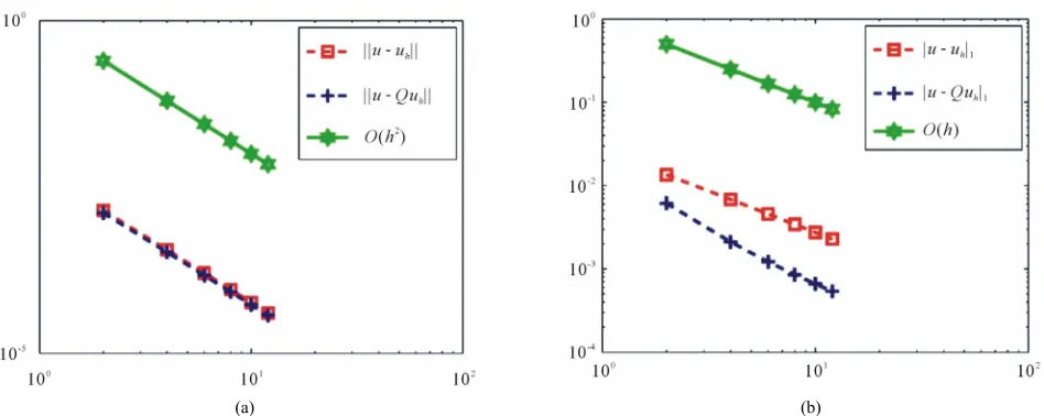
Figure 1. (a) Convergence rate of L2-norm error; (b) Convergence rate of H1-norm error.
(a) (b)
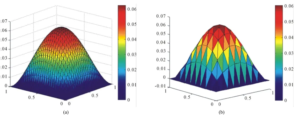
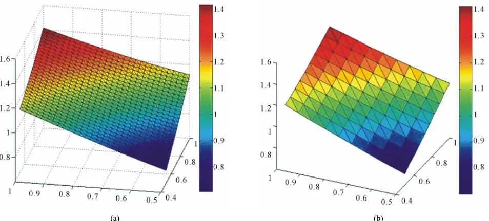
Figure 2. (a) Surface plot of approximation solution uh; (b) Surface plot of approximation solution Qτuh.
[image:2.595.54.544.344.711.2] [image:2.595.62.543.529.716.2]
From the results shown in Table 2, it is clear that the exact solution u in H1-norm has the superconvergence, but there is no improvement in the L2-norm, see Figures 3(a) and (b). The finite element solution given in Fig-ures 4(a) and (b). This agrees well with the theory.
Example 3.3: Let the domain
0,1 0,1 and the exact solution is assumed as
cos π
. 2
x y
u
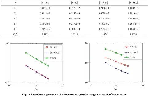
Table 3 gives the errors profile for Example 3. Notice that, the gradient estimate is of order
1.3 , that isO h
much better than the optimal order . Although, there is no improvement in the L2-norm, see Figure 5.
O hFigure 6 shows that the approximation solutions
and . h
u
h
Also, our numerical results and theoretical conclusions in Theorems (2.1) and (2.2) show highly consistent.
[image:3.595.58.538.220.514.2]Q u
Table 2.Errors on uniform triangular meshesThand Tτ.
h uuh1 uuh uQuh1 uQuh
2−3 0.9629e−1 0.1598e−2 0.2242e−1 0.1498e−2
3−3 0.4063e−1 0.2850e−3 0.6872e−2 0.2669e−3
4−3 0.2080e−1 0.7475e−4 0.2810e−2 0.6998e−4
5−3 0.1204e−1 0.2503e−4 0.1359e−2 0.2343e−4
6−3 0.7582e−2 0.9929e−5 0.7363e−3 0.9294e−5
O h 0.9998 1.9991 1.3427 1.9995
(a) (b)
Figure 3. (a) Convergence rate of error L2-norm error; (b) Convergence rate of H1-norm error.
(a) (b)
[image:3.595.61.542.527.715.2]Table 3. Errors on uniform triangular meshes Thand Tτ.
h uuh1 uuh uQuh1 uQuh
2−3 0.9135e−1 0.1770e−2 0.2150e−1 0.1689e−2
3−3 0.3855e−1 0.3157e−3 0.6579e−2 0.3010e−3
4−3 0.1973e−1 0.8278e−4 0.2692e−2 0.7893e−4
5−3 0.1142e−1 0.2772e−4 0.1303e−2 0.2643e−4
6−3 0.7193e−2 0.1099e−4 0.7062e−3 0.1048e−4
O h 0.9999 1.9993 1.3424 1.9994
(a) (b)
Figure 5. (a) Convergence rate of L2-norm error; (b) Convergence rate of H1-norm error.
(a) (b)
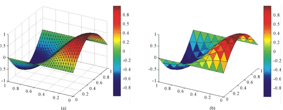
Figure 6. (a) Surface plot of approximation solution uh; (b) Surface plot of approximation solution Qτuh.
4. Superconvergence by Local
L
2-Projection
Notice that, the exact solution u may be not smooth globally on in practical computation, although the solution might be smooth enough locally for a good su-per convergence.
To this end, let 0 be a subdomain of where the exact solution u is sufficiently smooth. Let 1 be an-
other subdomain of such that 0 1. Define fi-nite element space The L2-projection
2 1
s
V H
Q from L2
onto the finite element space V is said to be local L2-projection.The following theorem can be found in [1].
Theorem 4.1: Assume that 1 s k 1 and the finite element space 2
0
s
V H . If the exact solution
1 1
0
k r
H H
1
,g
[image:4.595.56.545.205.593.2] [image:4.595.67.541.420.602.2]constant C such that
0 0
0 0
( 1) ,
h h
r
h
u Q u h u Q u
Ch u Ch u u
where h is the finite element approximation of (1)-(2). Theorem 4.2: Suppose that 1
u
1 s k
. Let the sur- face fitting spaces V Hs2
0 and uh be the finiteelement approximation of (1)-(2). Then, the post-proc- essing of uh is estimated by
1
.1 min 0, 2 k s
r s
5. Numerical Experiments for Local
L
2-Projection
In this section, we present several numerical experiments to verify the theoretical analysis in [1]. The triangulation is constructed by: 1) dividing the domain into an
h
T
3
n n3 rectangular mesh; 2) connecting the diagonal line with the positive slope. Denote h 13
n
as the mesh size.
The finite element space is defined by
11
; ; , on .
h g K h
V v H v P K K T vg
We define V as follows:
2
2
: K ;
V v L v P K K T .
Example 5.1: Let the domain
0,1 0,1 and
0 0, 0.5 0, 0.5
. The exact solution is assumed as 1 . 2 u x y
It is clear that the exact solution u is singular and f blows down at the boundary of
0,1 0,1 , seeFigure 7, however, h and Q u h are sufficiently smooth
on
u
0,1 0,1 , see Figure 8.
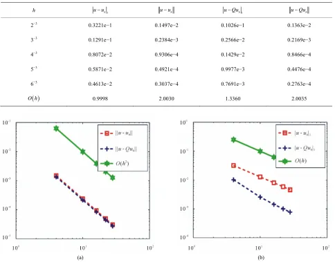
Table 4 shows that after the post-processing method, all the errors are reduced. The exact solution in L2-norm of u Q u h has the similar convergence rate as
h
u u which is shown as . There is no im- provement for the u in L2-norm. However, the error in H1-norm have higher convergence rate, which is shown
2O h
as
1.3O h for
u Q u h
. The order of conver-gence rate is O h
0.3 better than
h u uh
, see Figure 9.
Example 5.2: Let the domain 0,1 0,1 and
0 0.5,1 0.5,1
. The exact solution is assumed as
2 2
u x y
Obviously, the exact solution has singularity on the origin at the domain
0,1 0,1 , see Figure 10(a). On the same domain the function f blows down at the boundary, see Figure 10(b). The approximation solu- tions u and have been plot in the proper subdo-main h
Q u
0
From the results shown in Table 5, it is clear that the exact u in H1-norm has the superconvergence, but there is no improvement in the L2-norm, see Figure 12. This agrees well with the theory.
0.5,1 0.5,1
, see Figure 11.
Example 6: Let the domain
0,1 0,1 and
0 0.5,1 0.5,1
. The exact solution is assumed as
2 2.
y u
x y
From Figures 13(a) and (b), respectively observe that the exact solution has strongly singularity on the origin of the domain
0,1 0,1h
u Q u h
and the function f blows up at the boundary, Figure 14 show how the approxima-tion soluapproxima-tion and look like at the proper sub-domain 0
0.5,1
0.5,1
.
(a) (b)
(a) (b)
[image:6.595.63.542.85.295.2]Figure 8. (a) Surface plot of approximation solution uh; (b) Surface plot of approximation solution Qτuh. Table 4. Errors on uniform triangular meshes Thand Tτ.
h uuh1 uuh uQuh1 uQuh
2−3 0.3221e−1 0.1497e−2 0.1026e−1 0.1363e−2
3−3 0.1291e−1 0.2384e−3 0.2566e−2 0.2169e−3
4−3 0.8072e−2 0.9306e−4 0.1429e−2 0.8466e−4
5−3 0.5871e−2 0.4921e−4 0.9977e−3 0.4476e−4
6−3 0.4613e−2 0.3037e−4 0.7691e−3 0.2763e−4
O h 0.9998 2.0030 1.3360 2.0035
(a) (b)
[image:6.595.57.541.338.717.2]
(a) (b)
Figure 10. (a) Surface plot of exact solution u; (b) f blows down at the boundary.
(a) (b)
[image:7.595.60.540.85.300.2]Figure 11. (a) Surface plot of approximation solution uh; (b) Surface plot of approximation solution Qτuh. Table 5. Errors on uniform triangular meshes Thand Tτ.
h uuh1 uuh uQuh1 uQuh
2−3 0.1352e−1 0.1400e−2 0.6141e−2 0.1287e−2
3−3 0.6835e−2 0.3596e−3 0.2110e−2 0.3314e−3
4−3 0.4566e−2 0.1607e−3 0.1215e−2 0.1481e−3
5−3 0.3427e−2 0.9058e−4 0.8529e−3 0.8352e−4
6−3 0.2743e−2 0.5802e−4 0.6590e−3 0.5350e−4
[image:7.595.61.538.329.545.2] [image:7.595.58.543.591.731.2]
(a) (b)
Figure 12. (a) Convergence rate of L2-norm error; (b) Convergence rate of H1-norm error.
(a) (b)
Figure 13. (a) Surface plot of exact solution u; (b) f blows up at the boundary.
(a) (b)
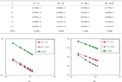
[image:8.595.62.536.87.276.2] [image:8.595.62.540.303.496.2] [image:8.595.50.538.321.709.2]Table 6. Errors on uniform triangular meshes Thand Tτ.
h uuh1 uuh uQuh1 uQuh
2−3 0.1186e−1 0.4006e−3 0.4708e−2 0.2779e−3
3−3 0.5979e−2 0.1009e−3 0.1621e−2 0.6959e−4
4−3 0.3992e−2 0.4490e−4 0.9518e−3 0.3094e−4
5−3 0.2996e−2 0.2527e−4 0.6760e−3 0.1740e−4
6−3 0.2397e−2 0.1617e−4 0.5261e−3 0.1113e−4
O h 0.9943 1.9949 1.3304 1.9989
(a) (b)
Figure 15. (a) Convergence rate of L2
-norm error; (b) Convergence rate of H1
-norm error.
Table 6 gives the errors profile for Example 6. Notice that, the gradient estimate is of order
1.3 that isO h
much better than the optimal order . Although, there is no improvement in the L2-norm, see Figure 15. Also, the numerical results and theoretical conclusions show highly consistent.
O hREFERENCES
[1] J. Wang, “A Superconvergence Analysis for Finite Ele-ment Solutions by the Least-Squares Surface Fitting on Irregular Meshes for Smooth Problems,” Journal of Mathematical Study, Vol. 33, No. 3, 2000, pp. 229-243. [2] R. E. Ewing, R. Lazarov and J. Wang,
“Superconver-gence of the Velocity along the Gauss Lines in Mixed Fi-nite Element Methods,” SIAM Journal on Numerical Analysis, Vol. 28, No. 4, 1991, pp. 1015-1029.
doi:10.1137/0728054
[3] M. Zlamal, “Superconvergence and Reduced Integration
in the Finite Element Method,” Mathematics Computa-tion, Vol. 32, No. 143, 1977, pp. 663-685.
doi:10.2307/2006479
[4] L. B. Wahlbin, “Superconvergence in Galerkin Finite Element Methods,” Lecture Notes in Mathematics, Springer, Berlin, 1995.
[5] A. H. Schatz, I. H. Sloan and L. B. Wahlbin, “Supercon-vergence in Finite Element Methods and Meshes that Are Symmetric with Respect to a Point,” SIAM Journal on Numerical Analysis, Vol. 33, No. 2, 1996, pp. 505-521. doi:10.1137/0733027
[6] M. Krizaek and P. Neittaanmaki, “Superconvergence Phenomenon in the Finite Element Method Arising from Avaraging Gradients,” Numerische Mathematik, Vol. 45, No. 1, 1984, pp. 105-116.