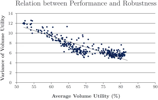
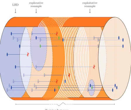
Tuning the Parameters of a Loading Algorithm

Source separation and kerbside collection make it possible to separate about 50% of the mixed waste for energy use and direct half of the waste stream to material recovery

I understand that I will be permitted to write an unlimited number of checks against my Account balance and that funds will be drawn in the following order: (1) against any

Walaupun pada kadar masukan berbeza, butiran enapcemar aerobik telah berjaya dibentuk untuk perawatan air sisa berkadaran tinggi

Goldfish care Planning your aquarium 4-5 Aquarium 6-7 Equipment 8-11 Decorating the aquarium 12-15 Getting started 16-17 Adding fish to the aquarium 18-19 Choosing and

Todavia, nos anos 1800, essas práticas já não eram vistas com tanta naturalidade, pelos menos pelas instâncias de poder, pois não estava de acordo com uma sociedade que se

Area Custodial Coordinators 5 FTE Custodial Staff 14 FTE Custodial Services Administrator 1 FTE Director of Maintenance 2 FTE Environmental Programs 9 FTE Energy Management 2

La formación de maestros investigadores en el campo del lenguaje y más específicamente en la adquisición de la escritura en educación ini- cial desde una perspectiva

For the poorest farmers in eastern India, then, the benefits of groundwater irrigation have come through three routes: in large part, through purchased pump irrigation and, in a