WORKING PAPERS SERIES
WP04-18
Testing for One-Factor Models versus
Stochastic Volatility Models
Testing for One-Factor Models versus Stochastic Volatility Models
∗Valentina Corradi†
Queen Mary, University of London
Walter Distaso‡ University of Exeter
November 2004
Abstract
This paper proposes a testing procedure in order to distinguish between the case where the volatility of an asset price is a deterministic function of the price itself and the one where it is a function of one or more (possibly unobservable) factors, driven by not perfectly correlated Brownian motions. Broadly speaking, the objective of the paper is to distinguish between a generic one-factor model and a generic stochastic volatility model. In fact, no specific assumption on the functional form of the drift and variance terms is required.
The proposed tests are based on the difference between two different nonparametric estimators of the integrated volatility process. Building on some recent work by Bandi and Phillips (2003) and Barndorff-Nielsen and Shephard (2004a), it is shown that the test statistics converge to a mixed normal distribution under the null hypothesis of a one factor diffusion process, while diverge in the case of multifactor models. The findings from a Monte Carlo experiment indicate that the suggested testing procedure has good finite sample properties.
Keywords: realized volatility, stochastic volatility models, one-factor models, local times, occupation densities, mixed normal distribution
JEL classification: C22, C12, G12.
∗We are grateful to Karim Abadir, Carol Alexander, James Davidson, Marcelo Fernandes, Nour Meddahi, Peter
Phillips and the seminar participants to the 2004 SIS conference in Bari, University of Exeter and Universit`a di
Padova for very helpful comments and suggestions. The authors gratefully acknowledge financial support from the ESRC, grant code R000230006.
†Queen Mary, University of London, Department of Economics, Mile End, London, E14NS, UK, email:
‡University of Exeter, Department of Economics, Streatham Court, Exeter EX4 4PU, UK, email:
1
Introduction
In finance the dynamic behavior of underlying economic variables and asset prices has been often described using one-factor diffusion models, where volatility is a deterministic function of the level of the underlying variable.1
Since determining the functional form of such diffusion processes is particularly important for pricing contingent claims and for hedging purposes, several specification tests have been proposed, within the class of one-factor models.
Examples include A¨ıt-Sahalia (1996), who compares the parametric density implied by a given null model with a nonparametric kernel density estimator. He rejects most of the commonly employed models and argues that rejections are mainly due to nonlinearity in the drift term.2 Similar findings to those of A¨ıt-Sahalia (1996) have been also provided by Stanton (1997) and Jiang (1998). Durham (2003) also rejects most of the popular models; in his case rejections are mainly due to misspecification of the volatility term. In particular, he finds implausibly high values for the elasticity parameter in the Constant Elasticity of Variance (CEV) model, implying violation of the stationarity assumption. Bandi (2002) applies fully nonparametric estimation of the drift and variance diffusion terms, based on the spatial methodology of Bandi and Phillips (2003), and finds that the drift term is very close to zero over most of the range of the short term interest rate. Therefore, rejections of a given model seem to be due to failure of the mean reversion property rather than to nonlinearity in the drift term. Qualitatively similar findings are obtained by Conley, Hansen, Luttmer and Scheinkman (1997), using generalized method of moments tests based on the properties of the infinitesimal generator of the diffusion.3
Most of the papers cited above have suggested testing and modeling procedures which are valid under the maintained hypothesis of a one-factor diffusion data generating process. Hence, the need of testing for the validity of the whole class of one-factor models.
This is the objective of the paper. Under minimal assumptions, the paper proposes a testing procedure in order to distinguish between the case in which the volatility process is a deterministic function of the level of the underlying variable and the one in which it is a function of one or more
1Although in the financial literature there is a somewhat widespread consensus about the fact that stock prices are better characterized by multifactor stochastic volatility models, short term interest rates are still often modeled as a one-factor diffusion process, in which volatility is a deterministic function of the level of the variable (see e.g.
Vasicek, 1977, Brennan and Schwartz, 1979, Cox, Ingersoll and Ross, 1985, Chan, Karolyi, Longstaffand Sanders, 1992, Pearson and Sun, 1994).
2A¨ıt-Sahalia (1996) does not reject a generalized version of the Constant Elasticity of Variance model. His results have been revisited by Pritsker (1998), who points out the sensitivity of A¨ıt-Sahalia’s test to the degree of dependency
in the short interest rate process.
(possibly unobservable) factors, driven by not perfectly correlated Brownian motions. With a slight abuse of terminology, the former class of models is referred to as one-factor models and the latter as stochastic volatility models.4 In particular, the paper compares generic classes of one-factor versus stochastic volatility models, without making assumptions on the functional forms of either the drift or the variance component.
If the null hypothesis is not rejected, then one can use the different testing and modeling pro-cedures mentioned above, based on the maintained hypothesis of a one-factor diffusion generating process. Conversely, if the null hypothesis is rejected, then one has to perform model diagnostics within the class of stochastic volatility models, using for example the efficient method of moments (e.g. Chernov, Gallant, Ghysels and Tauchen, 2003), or generalized moment tests based on the properties of the infinitesimal generator of the diffusion (see e.g. Corradi and Distaso, 2004). For example, one can test the validity of multi factor term structure models, suggested by e.g. Duffie and Singleton (1997), Dai and Singleton (2000, 2002).
The suggested test statistics are based on the difference between a kernel estimator of the instantaneous variance, averaged over the sample realization on a fixed time span, and realized volatility. The intuition behind the chosen statistic is the following: under the null hypothesis of a one-factor model, both estimators are consistent for the underlying integrated volatility; under the alternative hypothesis the former estimator is not consistent, while the latter is. More precisely, building on some recent work by Bandi and Phillips (2003) and Barndorff-Nielsen and Shephard (2004a), it is shown that the statistics weakly converge to mixed normal distributions under the null hypothesis and diverge at an appropriate rate under the alternative. The derived asymptotic theory is based on the time interval between successive observations approaching zero, while the time span is kept fixed. As a consequence, the limiting behavior of the statistic is not affected by the drift specification. Also, no stationarity or ergodicity assumption is required.
The proposed testing procedure is derived under the assumptions that the underlying variables are observed without measurement error and that the generating processes belong to the class of continuous semimartingales. Therefore, the provided tests are not robust to the presence of either jumps or market microstructure effects; more precisely, when either of the two occur, the test tends to reject the null hypothesis, even if the volatility process is a deterministic function of the underlying variable. However, as the test is computed over a finite time span, one can first test for the hypotheses of no jumps and no microstructure effects, and then perform the suggested testing procedure over a time span in which neither of the hypotheses above is rejected.
The rest of this paper is organized as follows. In Section 2, the testing procedure is outlined and the relevant limit theory is derived. Section 3 reports the findings from a Monte Carlo exercise, in order to assess the finite sample behavior of the proposed tests. Concluding remarks are given in Section 4. All the proof are gathered in the Appendix.
In this paper,−→p ,−→d and −→a.s. denote respectively convergence in probability, in distribution
and almost sure convergence. We write 1{·} for the indicator function, $!% for the integer part of
!,IJ for the identity matrix of dimensionJ and Z ∼MN (·,·) to denote that the random variable
Z is distributed as a mixed normal.
2
Testing for One-Factor vs Stochastic Volatility Models
2.1 Set-Up
As discussed above, our objective is to device a data driven procedure for deciding between one-factor diffusion models and stochastic volatility models, under minimal assumptions.
We consider the following class of one-factor diffusion models
dXt = µ(Xt)dt+σtdW1,t
σt = σ(Xt) (1)
and the following class of stochastic volatility models
dXt = µ(Xt)dt+σtdW1,t
σ2t = g(ft)
dft = b(ft)dt+σ1(ft)dW2,t, (2)
whereftis typically an unobservable state variable driven by a Brownian motion,W2,t, possibly but
not perfectly correlated with the Brownian motion drivingXt, thus allowing for possible leverage
effects.
The models in (1) encompass the class of parametric specifications analyzed by A¨ıt-Sahalia (1996), and they also allows for generic nonlinearities. The models in (2) include the square root stochastic volatility of Heston (1993), the Garch diffusion model (Nelson, 1990), the lognormal stochastic volatility model of Hull and White (1987) and Wiggins (1987), and are also related to the class of eigenfuction stochastic volatility models of Meddahi (2001). Note that ft may be a
multidimensional process, thus allowing for multifactor stochastic volatility processes. Also, the one-factor model may be possibly nested within the stochastic volatility model, in the sense that we can allow for the specification σ2
propose to extend the different one-factor models by adding a stochastic volatility term, and suggest models in which volatility depends on both the level of the underlying variable and a latent factor, driven by a different Brownian motion.5
In particular, it should be stressed that in our procedure we compare generic classes of one factor versus stochastic volatility models, without any functional form assumption on either the drift or the variance term.
We state the hypothesis of interest as
H0:σ2t =σ2(Xt), a.s.
versus the alternative
HA:σt2 =g(ft), a.s.
where ∀ω ∈ Ω+,!!!"1
0 (g(fs)−g(Xs)) ds
! !
! )= 0 and Pr (Ω+) = 1, with Ω+ ∈ Ω, and Ω denotes the probability space on which (ft, Xt) are defined.
Thus, under the null hypothesis the volatility process is a measurable function of the return processXt.On the other hand, under the alternative, the volatility process is a measurable function
of a possibly unobservable processft.In the paper, we simply require that the occupation densities
of the observable processXtand of the (possibly) unobservable factorftdo not coincide. In fact, if
they do coincide, then the integrated volatility process would be almost surely the same under both hypotheses. Finally, note that the case ofσ2
t =σ2(Xt)g(ft) falls under the alternative hypothesis,
while the case of a constant variance falls under the null.
In the sequel, we assume that we have data recorded at two different frequencies, over a fixed time span, which for sake of simplicity, but without loss of generality, is assumed equal to 1.6 More specifically, we assume to have n and m observations, with m ≤n, so that the discrete sampling
interval is equal respectively to 1/n and 1/m.
The proposed test statistics are based on
Zn,m,r=√m
1
n
!(n%−1)r#
i=1
Sn2(Xi/n)−RVm,r
, (3)
wherer ∈(0,1],
Sn2(Xi/n) =
(n−1
j=1 1{|Xj/n−Xi/n|<ξn}n )
X(j+1)/n−Xj/n
*2
(n−1
j=11{|Xj/n−Xi/n|<ξn}
(4)
5Andersen and Lund (1997) find that the inclusion of a stochastic volatility component in a square root model helps the elasticity parameter to fall in the stationary region. Durham (2003) finds that, although the addition of a
second factor increases the likelihood, it has very little impact as to what concerns bond pricing.
and
RVm,r =
!(m%−1)r#
j=1
)
X(j+1)/m−Xj/m
*2
. (5)
Note thatS2
n(Xi/n) is a nonparametric estimator of the volatility process evaluated atXi/n;
Florens-Zmirou (1993) has established consistency and the asymptotic distribution of a scaled version of (4) when the variance process follows (1).7 Recently,S2
n(Xi/n) has been used by Bandi and Phillips
(2003), in the context of fully nonparametric estimation of diffusion processes; their asymptotic theory is based on both the time span going to infinity and the discrete interval between successive observations going to zero. This is because they are interested in the joint estimation of the drift and variance diffusion terms.8
Conversely, our objective is to distinguish between the cases in which volatility is a measurable function of the observable process, and the one in which it depends on some other state variable. Therefore we remain silent about the drift term, and we only consider asymptotic theory in terms of the discrete interval approaching zero. In fact, on a finite time span the contribution of the drift term is asymptotically negligible.
Notice thatS2
n(Xi/n) is a consistent estimator of the instantaneous variance only under the null
hypothesis. Therefore, also its average over the sample realization of the process on a finite time span, 1/n(!i=1(n−1)r#S2
n(Xi/n), is a consistent estimator of integrated volatility only under the null
hypothesis.
RVm,r, which is known as realized volatility, has been proposed as a measure for volatility
concurrently by Andersen, Bollerslev, Diebold and Labys (2001), Andersen, Bollerslev, Diebold and Ebens (2002) and Barndorff-Nielsen and Shephard (2002). The properties of realized volatility have been extensively analyzed by Barndorff-Nielsen and Shephard (2002, 2004a,b), Andersen, Bollerslev, Diebold and Labys (2003), Barndorff-Nielsen, Graversen and Shephard (2004) (see also Andersen, Bollerslev, Meddahi, 2004a,b, and Meddahi, 2002, 2003). Realized volatility is a “model free” estimator of the quadratic variation of the processes defined in (1) and (2), and is consistent for the integrated (daily) volatility under both hypotheses. Barndorff-Nielsen and Shephard (2004a) have shown that a scaled and centered version of RVm,r weakly converges to a mixed normal
distribution when the log price process follows a continuous semimartingale, a result which we will use in the proof of our Theroem 1. The reason why we use two different sample frequencies in the
7The estimatorS2
n(Xi/n)has been also used by Corradi and White (1999) in order provide a test for the correct specification of the variance process, regardless of the drift specification. Within the class of one-factor models, a more general test, also allowing for time non-homogeneity, has been suggested by Dette, Podolskij and Vetter (2004).
8Bandi and Phillips (2003) consider a slightly modified version ofS2
computation ofSn2(Xi/n) andRVm,r will become clear in the next subsection.
In the sequel we shall need the following assumption.
Assumption 1.
(a) σ(·) and µ(·), defined in (1), satisfy local Lipschitz and growth conditions. Therefore, for any compact subsets M (under the null hypothesis) and J (under the alternative hypothesis) of the range of the processXt, there exist constants K1M, K2M, K3M, K4M,K1J and K2J, such
that,∀(x, y)∈M and ∀(x$, y$)∈J,
|σ(x)−σ(y)|≤K1M|x−y|,
|σ(x)|2 ≤K2M(1 +|x|2),
|µ(x)−µ(y)|≤K4M|x−y|, !!µ(x$)−µ(y$)!!≤K2J|x$−y$|
and
xµ(x)≤K3M(1 +|x|2), x$µ(x$)≤K1J(1 +|x$|2).
(b) σ1(·) and b(·), defined in (2), satisfy local Lipschitz and growth conditions. Therefore, for
any compact subset L of the range of the process ft, there exist constants K1L, K2L, K3L and
K4L, such that, ∀(p, q)∈L,
|σ1(p)−σ1(q)|≤K1L|p−q|, |σ1(p)|2 ≤K2L(1 +|p|2), |b(p)−b(q)|≤K3L|p−q| and
pb(p)≤K4L(1 +|p|2).
(c) µ(·),σ(·) and g(·) are continuously differentiable.
Assumption 1(a) states local Lipschitz and growth conditions for the drift term under both hy-potheses and for the variance term under the null hypothesis. Assumption 1(b) states local Lipschitz and growth conditions for the variance term under the alternative. Assumptions 1(a)(b) ensure the existence of a unique strong solution under both hypotheses (see e.g. Chung and Williams, 1990, p.229). Since we are studying the diffusion processes over a fixed time span, we do not need to impose more demanding assumptions, such as stationarity and ergodicity.9
2.2 Limiting Behavior of the Statistic
We can now establish the limiting distribution of the proposed test statistics based on Zn,m,r,
defined in (3), for both the cases where n=m and m/n→0,asm, n→ ∞.
Theorem 1. Let Assumption 1 hold.
Under H0,
(i)a if, as n, m,ξ−n1 → ∞, nξn → ∞ and for any arbitrarily small ε > 0, n1/2+εξn → 0, and if
m=n, then, pointwise in r ∈(0,1)
Zn,r −→d Zr ∼MN
+
0,2 , ∞
−∞
σ4(a)LX(r, a) (LX(1, a)−LX(r, a))
LX(1, a)
da
-, (6)
where Zn,r ≡Zn,n,r and
LX(r, a) = lim
ψ→0 1
ψ
1
σ2(a)
, r
0
1{Xu∈[a,a+ψ]}σ
2(X
u)du
denotes the standardized local time of the processXt.
(i)b Define Zn = maxj=1,...,J
! !Zn,rj
!
! and Z = maxj=1,...,J
! !Zrj
!
!, where 0 < r1 < . . . < rj−1 <
rj < . . . < rJ <1, for j = 1, . . . , J, with J arbitrarily large but finite. If, as n, m,ξn−1 → ∞,
nξn→ ∞, and, for any ε>0 arbitrarily small, n1/2+εξn→0, and ifm=n, then
Zn−→d Z,
with
Zr1 Zr2 ... ZrJ
∼MN 0,
V(r1, r1) V(r1, r2) . . . V(r1, rJ)
V(r2, r1) V(r2, r2) . . . V(r2, rJ)
... ... ... ... V(rJ, r1) V(rJ, r2) . . . V(rJ, rJ)
, (7)
where ∀r, r$,
V(r, r$) =V(r$, r) = 2 , ∞
−∞
σ4(a)LX(min(r, r
$), a) (L
X(1, a)−LX(min(r, r$), a))
LX(1, a)
da.
(i)c If, asn, m,ξn−1 → ∞,nξn→ ∞andnξ2n→0, and, for anyε>0arbitrarily small,m/n1−ε →
0,then
Zn,m,r−→d ZMr ∼MN
+
0,2 , ∞
−∞
σ4(a)LX(r, a)da
(i)d Define Zn,m = maxj=1,...,J
! !Zn,m,rj
!
! and ZM = maxj=1,...,J
! !ZMrj
!
!, where 0 < r1 < . . . <
rj−1 < rj < . . . < rJ < 1, for j = 1, . . . , J, with J arbitrarily large but finite. If, as
n, m,ξn−1 → ∞, nξn → ∞ and nξ2n→ 0, and, for any ε>0 arbitrarily small, m/n1−ε →0,
then
Zn,m −→d ZM,
with
ZMr1 ZMr2
... ZMrJ
∼MN 0,
V M(r1, r1) V M(r1, r2) . . . V M(r1, rJ)
V M(r2, r1) V M(r2, r2) . . . V M(r2, rJ)
... ... ... ...
V M(rJ, r1) V M(rJ, r2) . . . V M(rJ, rJ)
, (8)
where that, ∀r, r$,
V M(r, r$) =V M(r$, r) = 2 , ∞
−∞
σ4(a)LX(min(r, r$), a)da.
(ii) Under HA, if, as n, m,ξn−1 → ∞, nξn → ∞ and nξn2 → 0, and if m/n → π ≥ 0, then,
pointwise inr ∈(0,1],
Pr
+
ω: √1
m|Zn,m,r(ω)|≥ς(ω)
-→1,
where ς(ω)>0 for allω ∈Ω+, where Ω+ is defined as in the statement of H
A.
Notice that, as shown in the proof in the Appendix, under the alternative hypothesis, and in the case where ft is a one-dimensional process, the dominant term of the proposed statistic is
a scaled version of the absolute value of the difference between the local times of Xt and ft. If
instead ft is a multidimensional process, then the multivariate local time analogue of theLf(1, a)
used in Theorem 1 is not defined, but it can still be interpreted as a occupation density of the multivariate diffusion ft (see e.g. Geman and Horowitz, 1980 and Bandi and Moloche, 2001).
Therefore, in both cases, there exists an (almost surely) strictly positive random variable ς, such
that (1/√m)|Zm,n,r|≥ς,with probability approaching one.
The following Corollary considers the case where r = 1, i.e. when we use the whole span of
data in constructing the test statistic.
Corollary 1. Let Assumption 1 hold. Under H0, if, as n, m,ξ−n1 → ∞, nξn → ∞ and nξn2 → 0,
and, for any ε>0 arbitrarily small, m/n1−ε→0,then
Zn,m,1 −→d MN
+
0,2 , ∞
−∞
σ4(a)LX(1, a)da
Thus, for r= 1,the statistic has a mixed normal limiting distribution form/n→0 as m, n→ ∞.10
The theoretical results derived above provide an unfeasible limit theory, since the variance components have to be estimated. A consistent estimator of the standardized local time is given by
0
LX,n(r, a) =
1 2nξn
1
S2
n(a)
!(n%−1)r#
i=1 1{|X
i/n−a|<ξn}.
Thus an estimator of
2, ∞ −∞
σ4(a)LX(r, a) (LX(1, a)−LX(r, a))
LX(1, a)
da, (9)
i.e. of the quantity resulting in Theorem 1 part (i)a, is given by
, ∆2
∆1 0
σn4(a)
0
LX,n(r, a)
1 0
LX,n(1, a)−L0X,n(r, a)
2
0
LX,n(1, a)
da, (10)
where
0
σ4n(a) =
(n−1
i=1 1{|Xi/n−a|<ξn}n
2)X
(i+1)/n−Xi/n
*4
(n−1
i=1 1{|Xi/n−a|<ξn}
.
In order to implement the estimator in (10), we need to choose the interval of integration, ∆ = (∆1,∆2). Now, if we choose ∆ too small, then we may run the risk of getting an inconsistent estimator of the term in (9). On the other hand, if we choose ∆ too large, then for somea∈ ∆,
0
LX,n(r, a) andL0X,n(1, a) would be very close to zero, and the estimator in (10) will result in a ratio
of two terms approaching zero.
Of course, when computing (10) we can exclude alla∈∆for which, say,L0X,n(1, a)≤δn,where
δn→ 0 as n→ ∞.However, devicing a data-driven procedure for choosingδn is not an easy task.
In order to avoid this problem, we instead propose below an upper bound for the critical values of the limiting distribution in Theorem 1, parts (i)a and (i)b.
In fact, note that almost surely,
2, ∞ −∞
σ4(a)LX(r, a) (LX(1, a)−LX(r, a))
LX(1, a)
da
≤ 2
, ∞
−∞
σ4(a)LX(r, a)da≡2
, r
0
σ4(Xs)ds,
where the last equality above follows from Lemma 3 in Bandi and Phillips (2003). Now, Barndorff-Nielsen and Shephard (2002) have shown that
n
3
!(n%−1)r#
i=1
)
X(i+1)/n−Xi/n
*4 p
−→
, r
0
σ4sds, (11)
where σs4 = σ4(Xs) under H0 and σs4 =g2(fs) under HA; in other words the estimator defined in
(11) is consistent for the “true” integrated quarticity under both hypotheses and therefore provides an estimator of the upper bound of the term in (9).
On the other hand, we shall provide correct asymptotic critical values for the limiting distribu-tion in Theorem 1, parts (i)c and (i)d and in Corollary 1. In order to obtain asymptotically valid critical values and to make the limit theory derived in Theorem 1 part (i)d feasible, we will use a data-dependent approach. For s= 1, . . . , S, whereS denotes the number of replications, let
0 d(s)
m,r = 0 d(m,rs)1
0 d(m,rs)2
...
0 d(m,rs)J
= 0
Cm(r1, r1) C0m(r1, r1) C0m(r1, r1) C0m(r1, r1)
0
Cm(r1, r1) C0m(r2, r2) C0m(r2, r2) C0m(r2, r2) ... ... ... ...
0
Cm(r1, r1) C0m(r2, r2) . . . C0m(rJ, rJ)
1/2
η1(s)
η2(s)
...
ηJ(s)
, (12) where 0
Cm(rj, rj) =
2 3
!(m%−1)rj#
i=1
m)X(i+1)/m−Xi/m
*4
is a consistent estimator of twice the integrated quarticity and, for each s, 1η(1s)η2(s). . .ηJ(s)2$ is
drawn from a N(0,IJ). Then compute maxj=1,...,J
! ! !0d(m,rs)
! !
!,repeat this step S times, and construct
the empirical distribution. AsS→ ∞, the empirical distribution of maxj=1,...,J
! ! !0d(m,rs)
! !
!will converge
the distribution of a random variable defined as
max
j=1,...,J
! ! ! !MN
+
0,2 , ∞
−∞
σ4(a)LX(rj, a)da
-!!! !.
Therefore an asymptotically valid critical value for the limit theory in Theorem 1 part (i)d will be given byCVS
α, which denotes the (1−α)−quantile of the empirical distribution of maxj=1,...,J|d0(m,rs)j|,
computed usingS replications. Given the discussion above,CVαS will provide an upper bound for
the critical values of the limiting distribution derived in Theorem 1, part i(b). The implied rules for deciding between H0 and HAare outlined in the following Proposition.
Proposition 1. Let Assumption 1 hold.
(a) Let S → ∞. Suppose that as n, m,ξ−1
n → ∞, nξn→ ∞ and, for any ε>0 arbitrarily small,
n1/2+εξn→0. Ifm=n, then do not reject H0 if
Zn≤CVαS
(b) Let S → ∞. Suppose that, as n, m,ξn−1 → ∞, nξn → ∞ and nξn2 → 0 , and, for any ε>0
arbitrarily small, m/n1−ε→0; then do not reject H 0 if
Zn,m ≤CVαS
and reject otherwise. This rule provides a test with asymptotic size equal toαand asymptotic unit power.
As mentioned above, our test is designed to compare two classes of models, namely the one-factor diffusion models and the stochastic volatility models, regardless of the specification of the drift term. Therefore, if for example model (1) is augmented by adding another factor into the drift term (see e.g. Hull and White, 1994), our test will still fail to reject the null hypothesis considered, because the drift term is, over a fixed time span, of a smaller order of probability than the diffusion term and so is asymptotically negligible.
2.3 Market Microstructures and jumps
The asymptotic theory derived in the previous subsection relies on the fact that the underlying process is a continuous semi-martingale. However, some recent financial literature has pointed out the effects of possible jumps and market microstructure error on realized volatility (see e.g. Barndorff-Nielsen and Shephard, 2004c,d, Corradi and Distaso, 2004, Andersen, Bollerslev and Diebold, 2003 for jumps, and Sahalia, Mykland and Zhang, 2003, Zhang, Mykland and A¨ıt-Sahalia, 2003, Bandi and Russell, 2003, Hansen and Lunde, 2004 for microstructure noise).
We begin by analyzing the contribution of large and rare jumps. Suppose that the generating process in (1) is augmented by a jump component,
dXt=µ(Xt)dt+ dzt+σtdW1,t,
whereσt=σ(Xt),and zt is a pure jump process.
The test statistics based onZn,m,r are not robust to the presence of jumps. The intuitive reason
is that jumps have a different impact on the two components of the statistics, namely
n−1
!(n%−1)r#
i=1
Sn2(Xi/n) and RVm,r.
In fact, in the presence of jumps,RVm,r converges to the integrated volatility process plus the sum
of the squared magnitudes of the jumps (see Barndorff-Nielsen and Shephard, 2004c). Conversely,
n−1(!i=1(n−1)r#Sn2(Xi/n) converges to integrated volatility plus the weighted sum of the squared
jump occurring at time j/n has a larger effect on the componentn−1(i!=1(n−1)r#Sn2(Xi/n) if there
are many observations in the neighborhood ofXj/n.
However, since our test is carried over a fixed time span, we can pretest for the presence of no jumps, following for example Barndorff-Nielsen and Shephard (2004c,d); they proposed a test based on the properly scaled difference between realized volatility and bipower variation, which is a consistent estimator of integrated volatility in the presence of large and rare jumps in the log price process. If the null hypothesis is not rejected, we can apply our methodology. Huang and Tauchen (2004) also suggest a variety of Hausman type tests for jumps and find evidence of a relatively small number of jumps in the log price process. A similar finding is reported by Andersen, Bollerslev and Diebold (2003).
As for the presence of microstructure effects, suppose that the observed price of an asset can be decomposed into
Xj/m =Yj/m+,j/m.
Here ,j/m is interpreted as a noise capturing the market microstructure effect. The contribution
of the microstructure noise on realized volatility has already been analyzed in a series of recent papers (see e.g. A¨ıt-Sahalia, Mykland and Zhang, 2003, Zhang, Mykland and A¨ıt-Sahalia, 2003, Bandi and Russell, 2003 and Hansen and Lunde, 2004). For example, if the microstructure noise has a constant variance, i.e. independent of the sampling interval, then
m−1RVm,r −→p 2rν
where ν denotes the variance of the microstructure noise (see Zhang, Mykland and A¨ıt-Sahalia,
2003). As forn−1(!i=1(n−1)r#Sn2(Xi/n),due to the discreteness of the measurement error component,
the behavior of (nξn)−1(nj=1−11{|Xj/n−Xi/n|<ξn} is not easy to assess. Therefore, our procedure will
not be valid if the log price process is contaminated by microstructure noise.
Similarly to the case of large and rare jumps, it is possible to pretest the series under inves-tigation for the absence of microstructure noise. In fact, Awartani, Corradi and Distaso (2004) have suggested a simple test for the null hypothesis of no market microstructure, based on the appropriate scaled difference between two realized volatility measures constructed over different sampling frequencies.11 We can then apply our procedure over a time span for which neither the null hypothesis of no jumps nor the null hypothesis of no microstructure noise has been rejected.
11Awartani, Corradi and Distaso (2004) also propose a specification test of the null hypothesis of microstructure noise with constant variance. See also Barndorff-Nielsen and Shephard (2004c) for an alternative model of the market
3
A Simulation Experiment
In this section, the small sample performance of the testing procedure proposed in the previous section will be assessed through a Monte-Carlo experiment. Under the null hypothesis, we consider a version of the Cox, Ingersoll and Ross (1985) model with a mean reverting component in the drift,
dXt= (κ+µXt)dt+η
3
XtdW1,t. (13)
We first simulate a discretized version of the continuous trajectory of Xt under (13). We use
a Milstein scheme in order to approximate the trajectory, following Pardoux and Talay (1985), who provide conditions for uniform, almost sure convergence of the discrete simulated path to the continuous path, for given initial conditions and over a finite time span. In order to get a very precise approximation to the continuous path, we choose a very small time interval between successive observations (1/5760); moreover, the initial value is drawn from the gamma marginal distribution of Xt, and the first 1000 observations are then discarded.
We then sample the simulated process at two different frequencies, 1/nand 1/m, and compute
the different test statistics. In particular, the time span has been fixed to five days and five different values have been chosen for the number of intradaily observations n, ranging from 144
(corresponding to data recorded every ten minutes) to 1440 (corresponding to data recorded every minute). Therefore, the total number of observations ranges fromT n= 720 toT n= 7200, where T denotes the fixed time span expressed in days. Also, the experiment has been conducted for six
different values form(namely4)T n*.7/T5,4)T n*.75/T5,4)T n*.8/T5,4)T n*.9/T5,4)T n*.95/T5
and then the limiting case m=n). The process is repeated for a total of 10000 replications.
Results are reported for two test statistics, namely
Zn,m= max j=1,...,J
√
m ! ! ! ! ! !
1
n
!(n%−1)rj#
i=1
Sn2(Xi/n)−RVm,rj ! ! ! ! ! !
and
Zn,m,1=√m
6
1
n
n−1
%
i=1
Sn2(Xi/n)−RVm,1
7 .
Under the conditions stated in Theorem 1, we know that form/n→0,
Zn,m −→d ZM = max j=1,...,J
! !ZMrj
! !,
and for m=n,
Zn−→d Z = max j=1,...,J
! !Zrj
where the vectors (ZMr1ZMr2. . . ZMrJ)$ and (Zr1Zr2. . . ZrJ)$ are defined respectively in (8) and
(7). In the simulation experiment, J = 16, with r starting from r1 = .15 and then increasing by
.05 untilr16=.85. The critical values defined in (12) have been obtained withS = 1000. Similarly, under the conditions stated in Corollary 1, we have that form/n→0,
Zn,m,1−→d MN
+
0,2 , ∞
−∞
σ4(a)LX(1, a)da
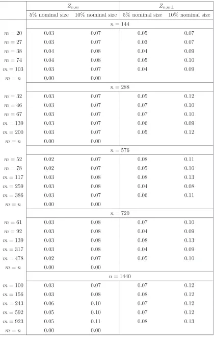
-The empirical sizes (at 5% and 10% level) of the tests discussed above are reported in Table 1, forκ= 0,η = 1,µ=−.8,ξn=n−10/13. The results for different values of the parameters needed to
generate (13) and the bandwidthξndisplay a virtually identical pattern and therefore are omitted
for space reasons. Inspection of the Table reveals an overall good small sample behaviour of the considered test statistics. The reported empirical sizes are everywhere very close to the nominal ones, with a slight tendency to underreject for the test based onZn,m. The zeros appearing in the
rows whenn=mare not surprising; in fact, when using the statisticZn, the critical values used in
the simulation exercise are just an upper bound of the true ones, and therefore one should expect an undersized test.
Under the alternative hypothesis, the following model has been considered,
dXt = (κ+µXt)dt+η
8
exp)σt2* 131−ρ2dW
1,t+ρdW2,t
2
dσt2 = (κ1+µ1σ2t)dt+η1
8
σ2tdW2,t. (14)
A discretized version of (14) has been simulated using a Milstein scheme as above, with κ1 = 1,
η1 = 1, µ1 = −.2. Then, using the obtained values of σt2, the series for Xt has been generated,
with ρ = 0 and keeping the remaining parameters at the values used to generate Xt under (13).
The findings for the power of the tests based on Zn,m and Zn,m,1 are reported in Table 2. The experiment reveals that the proposed tests has good power properties. The test based on Zn,m is
more powerful than the one based on Zn,m,1; this is not surprising, given that Zn,m is specifically
constructed to highlight the differences between the local times of Xt and ft. In fact, in the case
ofZm,n the term driving the power is maxr
! !"r
0 (LX(r, a)−Lf(r, a)) da
!
!,which is in general larger
than !!!"1
0 (LX(1, a)−Lf(1, a)) da
! !
!, the term driving the power of Zn. Also, the power of the test
based on Zn,m is generally increasing in n and m, as one should expect. In some cases, however,
the power remains constant or even decreases when m approaches n (namely, the cases when n= 144,288,576); this is due to the fact that, whenn =m, we are not using the correct critical
4
Concluding remarks
Table 1: Actual sizes of the tests based on Zn,m,r for different values of m and n
Zn,m Zn,m,1
5% nominal size 10% nominal size 5% nominal size 10% nominal size
n= 144
m= 20 0.03 0.07 0.05 0.07 m= 27 0.03 0.07 0.03 0.07 m= 38 0.04 0.08 0.04 0.09 m= 74 0.04 0.08 0.05 0.10
m= 103 0.03 0.07 0.04 0.09
m=n 0.00 0.00
n= 288
m= 32 0.03 0.07 0.05 0.12 m= 46 0.03 0.07 0.07 0.10 m= 67 0.03 0.07 0.07 0.10
m= 139 0.03 0.07 0.06 0.09
m= 200 0.03 0.07 0.05 0.12
m=n 0.00 0.00
n= 576
m= 52 0.02 0.07 0.08 0.11 m= 78 0.02 0.07 0.05 0.10
m= 117 0.03 0.08 0.08 0.13
m= 259 0.03 0.08 0.04 0.08
m= 386 0.03 0.07 0.06 0.11
m=n 0.00 0.00
n= 720
m= 61 0.03 0.08 0.07 0.10 m= 92 0.03 0.08 0.04 0.09
m= 139 0.03 0.08 0.08 0.13
m= 317 0.03 0.08 0.04 0.09
m= 478 0.02 0.07 0.05 0.10
m=n 0.00 0.00
n= 1440
m= 100 0.03 0.07 0.07 0.12
m= 156 0.03 0.08 0.08 0.12
m= 243 0.06 0.10 0.07 0.12
m= 592 0.05 0.10 0.07 0.12
Table 2: Actual powers of the tests based onZn,m,r for different values ofm and n
Zn,m Zn,m,1
5% nominal size 10% nominal size 5% nominal size 10% nominal size
n= 144
m= 20 0.12 0.22 0.14 0.17 m= 27 0.10 0.14 0.10 0.17 m= 38 0.14 0.18 0.09 0.15 m= 74 0.34 0.42 0.09 0.16
m= 103 0.38 0.44 0.19 0.25
m=n 0.42 0.44
n= 288
m= 32 0.20 0.26 0.11 0.21 m= 46 0.22 0.36 0.10 0.16 m= 67 0.44 0.48 0.12 0.16
m= 139 0.54 0.56 0.33 0.45
m= 200 0.56 0.64 0.26 0.30
m=n 0.54 0.54
n= 576
m= 52 0.22 0.26 0.11 0.16 m= 78 0.44 0.54 0.12 0.14
m= 117 0.48 0.54 0.16 0.19
m= 259 0.56 0.70 0.13 0.14
m= 386 0.84 0.88 0.70 0.76
m=n 0.76 0.82
n= 720
m= 61 0.44 0.52 0.12 0.18 m= 92 0.40 0.54 0.14 0.18
m= 139 0.58 0.66 0.21 0.25
m= 317 0.68 0.72 0.25 0.33
m= 478 0.72 0.82 0.22 0.29
m=n 0.76 0.88
n= 1440
m= 100 0.50 0.60 0.21 0.29
m= 156 0.55 0.75 0.20 0.24
m= 243 0.65 0.70 0.60 0.62
m= 592 0.90 0.90 0.88 0.89
A
Proofs
Before proving Theorem 1, we need the following Lemmas.
Lemma 1. Let Assumption 1 hold. Then
sup
s∈[0,1]|
µ(Xs)|=Oa.s.(nε/4),
sup
s∈[0,1]
! !σ2(Xs)
!
!=Oa.s.(nε/2),
sup
s∈[0,1]|
g(fs)|=Oa.s.(nε/2),
for anyε>0, arbitrarily small.
A.1 Proof of Lemma 1
We start from the case when Xt follows (1). Define Rl = {inf t : |Xt| > l}. Thus, Rl is an
Ft−measurable stopping time. Let
Xmin(t,Rl)= , min(
t,Rl)
0
µ(Xs)ds+
, min( t,Rl)
0
σ2(Xs)dW1,s.
Obviously, for allt≤Rl, Xmin(t,Rl) =Xt.Now let Ωl={ω :Rl>1}and l=ln=n
ε/4.Thus, given the growth conditions in Assumption 1(a),Xtis a non-explosive diffusion, and so Pr(Ωln →1) = 1.
By a similar argument, given Assumptions 1(a), 1(b), the same holds when the volatility process follows (2). Therefore, the statement follows. !
Lemma 2. Let Assumption 1 hold. Under H0, if, as n → ∞, nξn → ∞, nξn2 → 0 and, for any
ε>0 arbitrarily small, m/n1−ε→0, then, pointwise in r,
√
m n
!(n%−1)r#
i=1
)
Sn2(Xi/n)−σ2(Xi/n)*−→p 0.
A.2 Proof of Lemma 2
By Ito’s formula
√
m n
!(n%−1)r#
i=1
)
Sn2(Xi/n)−σ2(Xi/n)*
9 :; <
An,m,r
=
√
m n
!(n%−1)r#
i=1
(n−1
j=11{|Xj/n−Xi/n|<ξn}n )
X(j+1)/n−Xj/n*2 (n−1
j=1 1{|Xj/n−Xi/n|<ξn}
= √m
n
!(n%−1)r#
i=1
(n−1
j=11{|Xj/n−Xi/n|<ξn}2n
"(j+1)/n j/n
)
Xs−Xj/n
*
σ(Xs)dW1,s
(n−1
j=1 1{|Xj/n−Xi/n|<ξn}
9 :; <
Gn,m,r
+
√
m n
!(n%−1)r#
i=1
(n−1
j=11{|Xj/n−Xi/n|<ξn}2n
"(j+1)/n j/n
)
Xs−Xj/n
*
µ(Xs)ds
(n−1
j=11{|Xj/n−Xi/n|<ξn}
9 :; <
Hn,m,r
+
√
m n
!(n%−1)r#
i=1
(n−1
j=11{|Xj/n−Xi/n|<ξn}n
1"(j+1)/n j/n
)
σ2(Xs)−σ2(Xi/n)
*
ds2 (n−1
j=1 1{|Xj/n−Xi/n|<ξn}
9 :; <
Dn,m,r
. (15)
Thus, we need to show thatGn,m,r, Hn,m,r and Dn,m,r areoP(1).
Now, because of Lemma 1,
Dn,m,r ≤ √m sup
|Xs−Xτ|≤ξn !
!σ2(Xs)−σ2(Xτ)
! !
≤ √m sup
τ∈[0,1]
!
!∇σ2(Xτ)
!
! sup
|Xs−Xτ|≤ξn
|Xs−Xτ|
= O)√m*Oa.s.(nε/2)Oa.s(ξn) =oa.s.(1), (16)
provided that m1/2nε/2ξn→0.Since m=o(n1−ε), then
Oa.s(√mnε/2ξn) =oa.s(n1/2ξn),
which approaches zero almost surely.
As for Gn,m,r, by the proof of Step 1 of Theorem 1, part(i)a, below, (√n/√m)Gn,m,r = Gn,r
converges in distribution and so it’s OP(1); therefore Gn,m,r = oP(1), given that m/n → 0, as
m, n→ ∞.
Finally, given the continuity ofµ(·),
|Hn,m,r| ≤ √m sup s∈[0,1]|
µ(Xs)| sup
|i/n−s|≤1/n s∈[0,1]
!
!Xs−Xi/n
! !
= √mOa.s.(nε/4)Oa.s.
1
n−1/2logn2=oa.s.(1). (17)
In fact, because of the modulus of continuity of a diffusion (see McKean, 1969, p.96),
sup |i/n−s|≤i/n
s∈[0,1]
!
!Xs−Xi/n
!
!=Oa.s.
1
n−1/2logn2,
and n1/2−ε+ε/4n−1/2logn=n−3ε/4logn→0.Therefore, the statement follows. !
A.3 Proof of Theorem 1
(i)a
Zn,r = √1
n
!(n%−1)r#
i=1
)
Sn2(Xi/n)−σ2(Xi/n)*
9 :; <
An,r
−√n
!(n%−1)r#
j=1
)
X(j+1)/n−Xj/n
*2
−
, r
0
σ2(Xs)ds
9 :; <
Bn,r
+√1
n
!(n%−1)r#
i=1
σ2(Xi/n)−√n
, r
0
σ2(Xs)ds
9 :; <
Cn,r
. (18)
The proof of the statement is based on the four steps below.
Step 1: An,r −→d MN
1
0,2"−∞∞ σ4(a)LX(r,a)2
LX(1,a)da 2
.
Step 2: Bn,r−→d MN
1
0,2"−∞∞ σ4(a)LX(1, a)da
2 .
Step 3: Let < An, Bn>r define the discretized quadratic covariation process.
plimn→∞ < An, Bn>r−2
, ∞
−∞
σ4(a)LX(r, a)
2
LX(1, a)
da= 0.
Step 4: Cn,r=oP(1).
Proof of Step 1: First note that using Ito’s formula
An,r =
1
√
n
!(n%−1)r#
i=1
(n−1
j=1 1{|Xj/n−Xi/n|<ξn}n )
X(j+1)/n−Xj/n*2 (n−1
j=11{|Xj/n−Xi/n|<ξn}
−σ2(Xi/n)
= √1
n
!(n%−1)r#
i=1
(n−1
j=1 1{|Xj/n−Xi/n|<ξn}2n
"(j+1)/n j/n
)
Xs−Xj/n
*
σ(Xs)dW1,s
(n−1
j=11{|Xj/n−Xi/n|<ξn}
9 :; <
Gn,r
+√1
n
!(n%−1)r#
i=1
(n−1
j=11{|Xj/n−Xi/n|<ξn}2n
"(j+1)/n j/n
)
Xs−Xj/n
*
µ(Xs)ds
(n−1
j=1 1{|Xj/n−Xi/n|<ξn}
9 :; <
+√1
n
!(n%−1)r#
i=1
(n−1
j=11{|Xj/n−Xi/n|<ξn}n
1"(j+1)/n j/n
)
σ2(Xs)−σ2(Xi/n)
*
ds2 (n−1
j=1 1{|Xj/n−Xi/n|<ξn}
9 :; <
Dn,r
.
Now, given Lemma 1,Dn,r =oa.s.(1),provided thatn1/2+εξn→0,asn→ ∞.It is immediate
to see that Hn,r is of a smaller order of probability thanGn,r.
Let< Gn>rdenote the discretized quadratic variation process ofFn,r.By a similar argument
as in Bandi and Phillips (2003, pp.271-272),
plimn→∞ < Gn>r−2
, ∞
−∞
σ4(a)LX(r, a)
2
LX(1, a)
da= 0.
Thus, by the same argument as in the proof of Theorem 3 in Bandi and Phillips (2003), the statement in Step 1 follows.
Proof of Step 2: It follows from Theorem 1 in Barndorff-Nielsen and Shephard (2004a).
Proof of Step 3: The discretized covariation process< An, Bn>r,
< An, Bn>r
= 4n
!(n%−1)r#
i=1
!(n%−1)r#
j=1
1{|X
j/n−Xi/n|<ξn}
1"(j+1)/n j/n
)
Xs−Xj/n
*
σ(Xs)dWs
22
(n−1
j=1 1{|Xj/n−Xi/n|<ξn}
= 2n
!(n%−1)r#
i=1
!(n%−1)r#
j=1
1{|Xj/n−Xi/n|<ξn}σ
4(X
j/n+oa.s.(1))
(n−1
j=1 1{|Xj/n−Xi/n|<ξn}
(19)
= 2, r 0
6, r
0
1{|Xu−Xa|<ξn}σ
4(X
u)du
"1
0 1{|Xu−Xa|<ξn}du 7
da+oa.s.(1)
= 2, ∞ −∞
6, ∞
−∞
1{|u−a|<ξn}σ4(u)LX(r, u)du
"∞
−∞1{|u−a|<ξn}LX(1, u)du 7
LX(r, a)da+oa.s.(1),
where the 2 (instead of 4) on right hand side of (19) comes from Lemma 5.3 in Jacod and Protter (1998). Along the lines of Bandi and Phillips (2001, 2003), by the change of variable
u−a
ξn
=z,
we have that
= 2, ∞ −∞
6, ∞
−∞
1{|u−a|<ξn}σ
4(u)L
X(r, u)du
"∞
−∞1{|u−a|<ξn}LX(1, u)du 7
LX(r, a)da+oa.s.(1)
= 2, ∞ −∞
6, ∞
−∞
1{|zξn|<ξn}σ
4(a+zξ
n)LX(r, a+zξn)dz
"∞
−∞1{|zξn|<ξn}LX(1, a+zξn)dz 7
LX(r, a)da+oa.s.(1) a.s.
−→2
, ∞
−∞
σ4(a)LX(r, a)
2
LX(1, a)d
a. (20)
Proof of Step 4:
Cn,r = √1
n
!(n%−1)r#
i=1
σ2(Xi/n)−√n
, r
0
σ2(Xs)ds
= √1
n
!(n%−1)r#
i=1
σ2(Xi/n)−√n
!(n%−1)r#
i=1
, (i+1)/n i/n
σ2(Xs)ds
= √n
!(n%−1)r#
i=1
, (i+1)/n i/n
)
σ2(Xi/n)−σ2(Xs)
*
ds (21)
and, given the Lipschitz assumption on σ2(·), the last line in (21) is oP(1) by the same
argument as the one used in Step 1.
Given Steps 1-4 above, it follows that the quadratic variation process ofZn,r is given by
2, ∞ −∞
σ4(a)LX(r, a)da+ 2
, ∞
−∞
σ4(a)LX(r, a)
2
LX(1, a)d
a−4 , ∞
−∞
σ4(a)LX(r, a)
2
LX(1, a)d
a
= 2, ∞ −∞
σ4(a)LX(r, a) (LX(1, a)−LX(r, a))
LX(1, a)
da. (22)
The statement in the theorem then follows.
(i)b Without loss of generality, suppose thatr < r$.By noting that
1
√
n
!(n%−1)r#
i=1
Sn2(Xi/n)−√n
!(n%−1)r#
i=1
)
Xi+1/n−Xi/n
*2
= √1
n
[(n−1)r"]
%
i=1
Sn2(Xi/n)−√n
[(n−1)r"]
%
i=1
)
Xi+1/n−Xi/n
*2
,
with Sn2(Xi/n) = 0 and
)
Xi+1/n−Xi/n
*2 = 0 for
i > $(n−1)r%, the result then follows by
(i)c The statistic Zn,m,r can be rewritten as
Zn,m,r=
√
m n
!(n%−1)r#
i=1
)
Sn2(Xi/n)−σ2(Xi/n)
*
9 :; <
An,m,r
−√m
!(m%−1)r#
j=1
)
X(j+1)/m−Xj/m*2− , r
0
σ2(Xs)ds
9 :; <
Bm,r
+√m
n
!(n%−1)r#
i=1
σ2(Xi/n)−√m
, r
0
σ2(Xs)ds
9 :; <
Cn,m,r
. (23)
Note thatAn,m,r =oP(1) by Lemma 2.
We first need to show thatCn,m,r=oa.s.(1). Given Assumption 1(a), Lemma 1, and recalling
the modulus of continuity of a diffusion (see McKean, 1969, pp.95-96),
! ! ! ! ! ! √ m n
!(n%−1)r#
i=1
σ2(Xi/n)−√m
, r
0
σ2(Xs)ds
! ! ! ! ! ! = ! ! ! ! ! ! √ m n
!(n%−1)r#
i=1
σ2(Xi/n)−√m
!(n%−1)r#
i=1
, (i+1)/n i/n
σ2(Xs)ds
! ! ! ! ! ! = ! ! ! ! ! ! √ m
!(n%−1)r#
i=1
, (i+1)/n i/n
)
σ2(Xi/n)−σ2(Xs)
* ds ! ! ! ! ! !
≤ √m
!(n%−1)r#
i=1
, (i+1)/n i/n
!
!σ2(Xi/n)−σ2(Xs)
! !ds
≤ √m sup
|s−τ|≤1/n s∈[0,r]
!
!σ2(Xs)−σ2(Xτ)
!
!≤√m sup
τ∈[0,r]|∇
σ2(Xτ)| sup
|s−τ|≤1/n s∈[0,r]
|Xs−Xτ|
= √mOa.s.(nε/2)Oa.s.(n−1/2logn) =oa.s.(1),
asn1/2−ε/2n−1/2logn→0.Thus,
Zn,m,r =−Bm,r+oa.s.(1).
The statement then follows from the proof of Step 2 in part i(a).
(ii) We will prove the Theorem for the case analyzed in part (i)c; in the other cases the proof follows straightforwardly and is therefore omitted. Under HA, we have that
dXt = µ(Xt)dt+
8
σ2
tdW1,t
σt2 = g(ft)
dft = b(ft)dt+σ1(ft)dW2,t.
Pointwise in r,we can rewrite Zn,m,r as
Zn,m,r =
√
m n
!(n%−1)r#
i=1
)
Sn2(Xi/n)−g)fi/n**−√m
!(m%−1)r#
j=1
)
X(j+1)/m−Xj/m*2
+
√
m n
!(n%−1)r#
i=1
g)fi/n*
= √m
n
!(n%−1)r#
i=1
)
Sn2(Xi/n)−g)fi/n**
9 :; <
En,m,r
−√m
!(m%−1)r#
j=1
)
X(j+1)/m−Xj/m*2− , r
0
g(fs) ds
9 :; <
Fm,r
+
√
m n
!(n%−1)r#
i=1
g)fi/n*−√m , r
0
g(fs) ds
9 :; <
Ln,m,r
. (24)
By the same argument used in the proof of part (i)a, Step 4 and Step 2 (respectively)Ln,m,r=
oP(1) and Fm,r =OP(1).
We can expandEn,m,r as
En,m,r
=
√
m n
!(n%−1)r#
i=1
(n−1
j=1 1{|Xj/n−Xi/n|<ξn}n )
X(j+1)/n−Xj/n*2 (n−1
j=11{|Xj/n−Xi/n|<ξn}
−g)fi/n* = √ m n
!(n%−1)r#
i=1
(n−1
j=1 1{|Xj/n−Xi/n|<ξn}2n
"(j+1)/n j/n
)
Xs−Xj/n
* 3
g(fs)dW1,s
(n−1
j=11{|Xj/n−Xi/n|<ξn}
9 :; <