http://wrap.warwick.ac.uk
Original citation:He, Ligang, Jarvis, Stephen A., 1970-, Spooner, Daniel P. and Nudd, G. R.. (2004) Dynamic, capability-driven scheduling of DAG-based real-time jobs in heterogeneous cluster. International Journal of High Performance Computing and Networking (IJHPCN), Volume 2 (Number 2-4). pp. 165-177. ISSN 1740-0562
Permanent WRAP url:
http://wrap.warwick.ac.uk/61385
Copyright and reuse:
The Warwick Research Archive Portal (WRAP) makes this work by researchers of the University of Warwick available open access under the following conditions. Copyright © and all moral rights to the version of the paper presented here belong to the individual author(s) and/or other copyright owners. To the extent reasonable and practicable the material made available in WRAP has been checked for eligibility before being made available.
Copies of full items can be used for personal research or study, educational, or not-for profit purposes without prior permission or charge. Provided that the authors, title and full bibliographic details are credited, a hyperlink and/or URL is given for the original metadata page and the content is not changed in any way.
A note on versions:
The version presented here may differ from the published version or, version of record, if you wish to cite this item you are advised to consult the publisher’s version. Please see the ‘permanent WRAP url’ above for details on accessing the published version and note that access may require a subscription.
Dynamic, Capability-driven Scheduling of
DAG-based Real-time Jobs in Heterogeneous
Clusters
Ligang He, Stephen A. Jarvis, Daniel P. Spooner and Graham R. Nudd
Abstract—In this research a scenario is assumed where periodic real-time jobs are being run on a heterogeneous cluster of com-puters, and new aperiodic parallel real-time jobs, modelled by Directed Acyclic Graphs (DAG), arrive at the system dynami-cally. In the scheduling scheme presented in this paper, a global scheduler situated within the cluster schedules new jobs onto the computers by modelling their spare capabilities left by existing periodic jobs. Admission control is introduced so that new jobs are rejected if their deadlines cannot be met under the precondi-tion of still guaranteeing the real-time requirements of existing jobs. Each computer within the cluster houses a local scheduler, which uniformly schedules both periodic job instances and the subtasks in each parallel real-time job using an Early Deadline First policy. The modelling of the spare capabilities is optimal in the sense that once a new task starts running on a computer, it will utilize all the spare capability left by the periodic real-time jobs and its finish time will be the earliest possible. The performance of the proposed modelling and scheduling is evaluated through ex-tensive simulation; the results show that the system utilization is significantly enhanced, while the real-time requirements of the existing jobs remain guaranteed.
Index Terms—cluster computing, dynamic scheduling, spare capabilities, heterogeneous clusters, periodic real-time jobs, DAG real-time jobs, and performance prediction.
I. INTRODUCTION
luster systems are gaining in popularity for the processing of scientific and commercial applications [9]. The research has also taken place to extend conventional operating systems (such as Linux) to support real-time scheduling (e.g. preemp-tive scheduling using the Earliest-Deadline-First policy) [7], [23], and as a result cluster systems are increasingly used for the processing of applications with time constraints [1], [24]. Many scenarios about real-time processing can be represented abstractly, as the hybrid execution of both existing periodic jobs and newly arriving aperiodic jobs. An example of this is in
the reservation-based scheduling of multimedia applications, where the reservation of processor times can be expressed per period, so as to ensure that the processor utilization for an application is maintained above some required level [13]. These reserved executions can be viewed as periodic jobs and in addition to these the underlying processors also have to deal with other newly arriving jobs. This scenario presents the challenge of devising scheduling schemes which judicially deal with the hybrid execution of existing jobs (or reserved execu-tions) together with newly arriving jobs. This task is further complicated by trying to reduce the response times of newly arriving jobs while maintaining the time constraints of existing periodic jobs.
Manuscript received Dec 31, 2003. This work is sponsored in part by grants from the NASA AMES Research Center (administrated by USARDSG, con-tract no. N68171-01-C-9012), the EPSRC (concon-tract no. GR/R47424/01) and the EPSRC e-Science Core Programme (contract no. GR/S03058/01).
The authors are with the Department of Computer Science, University of Warwick, Coventry, CV4 7AL, United Kingdom. E-mail: {liganghe, saj, dps, grn}@dcs.warwick.ac.uk.
The dynamic scheduling technique presented in this paper addresses this issue, aiming to allocate newly arriving Aperi-odic Real-time Jobs (ARJ) to a heterogeneous cluster of com-puters on which Periodic Real-time Jobs (PRJ) are running. In this paper an ARJ is assumed to be a parallel job with time constraints, which is modeled as a real-time Directed Acyclic Graph (DAG) [15]. In this scheduling framework, a global scheduler - located on a computer in the heterogeneous cluster - analyzes the execution of PRJs on the remaining computers and models the initial distribution of their spare capabilities off-line. Once a new ARJ arrives at the system, the global scheduler releases the precedence constraints among the tasks in the ARJ, adjusts the initial distribution of spare capabilities (as this may have changed due to the execution of preceding ARJs) and then tries to place the execution of the tasks from the new ARJ into the spare time slots that are available. The re-sponse times of the tasks in the ARJ are computed, to determine whether the job can be accepted. If this is the case then the tasks in the ARJ will be sent to the designated computers and exe-cuted in parallel, exploiting the spare capabilities. Global scheduling for ARJs takes both task and message scheduling into account and local scheduling, at each computer, uses a uniform Early Deadline First (EDF) scheduling policy.
The modelling of spare capabilities proposed in this paper does not invoke any additional communication between the global scheduler and the remaining computers in the cluster. The approach is optimal in the sense that once a new task starts running on a computer, it will utilize all the spare capability left by the PRJs, and its finish time is the earliest possible. This work is supported by an existing Performance Analysis and
Characterization Environment (PACE) [14]. PACE can be used to predict application behavior and provide performance data (such as the execution time of a job) which supports the task of scheduling and resource management [6], [21].
The remainder of this paper is organized as follows: Section II presents the related work; Section III describes the workload and system model; in Section IV a novel approach is presented that allows a global scheduler to model the spare capabilities of computers in a cluster; Section V describes a global dynamic scheduling algorithm for DAG real-time jobs; a performance evaluation of this modelling approach and scheduling algo-rithm is presented in Section VI and Section VII concludes the paper.
II. RELATED WORK
The study of heterogeneous clusters or networks of work-stations has received a good deal attention [10], [11], [20], [25]. The scheduling of tasks with precedence constraints, which are usually represented by DirectedAcyclic Graphs (DAG), has also been well documented [2], [11], [15], [16], [26], [28], [30]. An off-line algorithm is presented in [2] to schedule commu-nicating tasks with precedence constraints in distributed sys-tems. However, the algorithm belongs to the static category. In [30] a dynamic incremental DAG scheduling approach for parallel machines is described. However, the approach is lim-ited to homogenous systems. Two low-complexity efficient heuristics, the Heterogeneous Earliest-Finish-Time Algorithm and the Critical-Path-on-a-Processor Algorithm are proposed in [28], each for the scheduling of DAGs on heterogeneous processors. These heuristics are not designed for real-time task allocation and are therefore not suitable for scheduling in a real-time context because job requirements cannot be guaran-teed. In [15] non-real-time DAGs are extended to include real-time information, and the scheduling of parallel tasks with real-time DAG topologies on heterogeneous systems is pro-posed. This technique differs from that presented in this paper because it is not aimed at the utilization of spare system capa-bilities.
A number of scheduling algorithms for periodic real-time jobs on multi-computer or multiprocessor systems have also been presented [3], [4], [17], [18]. A task duplication technique combined with pipelined execution for the scheduling of time critical periodic applications on heterogeneous systems can be found in [17]. In [3], a reward-based scheduling scheme for periodic tasks is presented. While these techniques are effec-tive, they are unable to deal with the hybrid execution of pe-riodic and apepe-riodic tasks.
Scheduling systems for the processing of both periodic and aperiodic real-time tasks can be classified into fixed or dynamic priority systems. Fixed priority systems assume that the priority of each periodic task is fixed, whereas in dynamic priority systems different instances of periodic tasks may have different priorities (such as in scheduling systems that use EDF). Dy-namic priority systems typically attain higher processor
utili-zation than fixed ones. Slack Stealing policies have been de-signed for fixed priority systems [12], while the Background (BG), Deadline Deferrable Server (DDS), Total Bandwidth Server (TBS) and Improved Priority Exchange (IPE) algo-rithms have been designed for dynamic priority systems [5], [19], [22], [29]. These techniques are widely used in embedded real-time systems, such as robot control systems. All these algorithms have been developed for uniprocessor architectures and aperiodic tasks are assumed to be independent and without precedence constraints. Techniques presented in [12] and [27] run aperiodic tasks by using the spare capabilities left by pe-riodic tasks; though in each case they are limited to uniproc-essor scenarios. [8] presents an algorithm to jointly schedule both periodic and aperiodic tasks on clusters. This however is not aimed at the exploitation of spare capabilities. In this same paper it is also assumed that aperiodic tasks are independent and non-real-time, that the cluster is homogeneous and that all periodic tasks start at the same time.
Extending the modelling of spare capabilities from uni-processor architectures to cluster environments is non-trivial. This is primarily because a uniprocessor system only needs to model the spare capabilities within itself, whereas in a cluster a central node models the spare capabilities of the other nodes in the system, making the information needed for this calculation far more difficult to attain. The modelling approach in this paper efficiently models the spare capabilities of computers in a heterogeneous cluster and significantly, is free of additional communication overheads. The proposed scheme is also de-signed for dynamic priority systems where an EDF policy is used for local scheduling.
III. WORKLOAD AND SYSTEM MODEL
A heterogeneous cluster of computers is modelled as P={p1, p2,..., pm}, where piis an autonomous computer. Each computer pi is weighted pwi, which represents the time it takes to perform one unit of computation. The computers in the heterogeneous cluster are connected by a multi-bandwidth local network. Each communication link between computer pi and pj, denoted by lij, is weighted lwij, which models the time it takes to transfer one message unit between pi and pj.
Each computer runs a set of PRJs, all of which are inde-pendent of one another. On a computer with n PRJs, the i-th periodic real-time job PRJi (1≤i≤n) is defined using the triple (Si, Ci, Ti), where Si is PRJi’s start time, Ci is PRJi’s execution time on the computer, and Ti is PRJi’s period (times are meas-ured in time units unless otherwise stated). An execution of
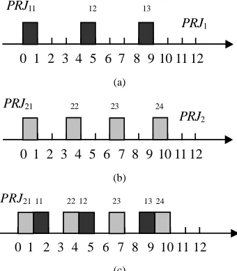
PRJi is called a Periodic Job Instance (PJI) and the j-th execu-tion is denoted by PJIij. PJIij is ready at time (j-1)*Ti, termed the ready time (Rij, Ri1=Si), and must be complete before j*Ti, termed the deadline (Dij). All PJIs must meet their deadlines and are scheduled using an EDF policy. Fig.1 shows two PRJs and their execution on a single computer; all the illustrations in this paper use these two PRJs as a working example.
accepted, an ARJ is run once. An ARJ is modelled as (avt, J), where avt is the ARJ’s arrival time and J defines the tasks and their topology in the ARJ. J={V, E}, where V={v1, v2,…, vr}, which defines the r real-time tasks that constitute the ARJ.
dt(vi) and cvi are denoted as vi’s deadline and computational volume; E represents the communication relationship and the precedence constraints among tasks; eij=(vi, vj)∈E represents a message sent from task vi to vj and it also states that vj will start to run only after vi is complete and vj receives message eij; vi is called vj’s predecessor and mvij is denoted as eij’s message volume.
PRJ1
0 1 2 3 4 5 6 7 8 9 10 11 12
PRJ11 12 13
(a)
0 1 2 3 4 5 6 7 8 9 10 11 12
PRJ21 22 23 24
PRJ2
(b)
0 1 2 3 4 5 6 7 8 9 10 11 12
PRJ2111 2212 23 1324
[image:4.612.87.257.193.387.2](c)
Fig. 1. A case study of PRJs (a) PRJ1 with a period of 4 and an execution time
of 1, (b) PRJ2 with a period of 3 and an execution time of 1, (c) execution of
PRJ1 and PRJ2 under EDF starting at 0
Fig.2 depicts the components of the scheduler model in the heterogeneous cluster environment. It is assumed that PRJs are active across computers, and a central computer in the cluster, the global scheduler, records Si, Ci and Ti for all PRJs. The global scheduler models the spare capacities left by the PRJs on the cluster.
S ched ulab le T asks Q ueue G lo b al S ched ule
Q ueue
• • •
G lobal S cheduler
Pm
P2
P1 L o cal S ched ule Q ueue
Local S ch ed u ler
Local S ch ed u ler
Local S ch ed u ler
P A C E
Fig. 2. The scheduler model in the heterogeneous cluster environment
All ARJs arrive at the global scheduler where they wait in a
global schedule queue. These new jobs are serviced on a First-Come-First-Served basis. Each time the global scheduler fetches a job from the head of the global schedule queue, it searches for schedulable tasks in the ARJ and inserts them into the schedulable task queue so that the deadlines of the tasks in the schedulable task queue are in increasing order.
The global scheduler then picks a task from the head of the schedulable task queue and schedules it globally. A task in an ARJ is considered schedulable if either the task has no
prede-cessors or all of its predeprede-cessors have been scheduled. A task is considered acceptable by a computer if it can be completed before its deadline and the real-time requirements of all the PRJs on that computer remain guaranteed. If a task is not ac-ceptable by any of the computers then it is rejected. Conse-quently, the ARJ that the task belongs to is rejected. When the global scheduler finishes scheduling a task, it searches for new schedulable tasks in the ARJ and updates the schedulable task queue. An ARJ is accepted if all its composite tasks are acceptable.
Once accepted, the tasks in the ARJ are sent to the local schedulers of the designated computers. At each computer, the local scheduler receives the new tasks and inserts them into a
local schedule queue, ensuring that the deadlines of the tasks (ARJ’s tasks or the PRJs’ PJIs) are in increasing order. The local scheduler uniformly schedules both the ARJs’ tasks and the PRJs’ PJIs using EDF. Each task to be executed is fetched from the head of the local schedule queue and the local sched-ule is preemptive.
In this scheduler model, PACE accepts ARJs, predicts the execution time of each task in the ARJs on each computer and then returns the predicted time to the global scheduler. After the global scheduler decides to schedule task vi on computer ps, assuming message eij=(vi, vj)∈E, PACE is called to predict eij’s communication time on each link between ps and any other computer. In the current model it is assumed that the execution and communication times predicted by PACE are entirely ac-curate, and that the times for prediction, scheduling and task dispatching are negligible (extending the model is the subject of future work).
IV. SPARE CAPABILITY MODELLING
In this section, the initial distribution of idle time left by the PRJs (i.e. the spare capabilities left by the PRJs before certain time points) is modelled. This modelling procedure can be done off-line. The idle time distribution will be altered by the dy-namic arrivals of ARJs. Hence, an on-line mechanism is pre-sented for adjusting the initial idle time distribution when the global scheduler schedules a new arriving ARJ.
A. Off-line Modelling of the Initial Distribution of the Spare Capability
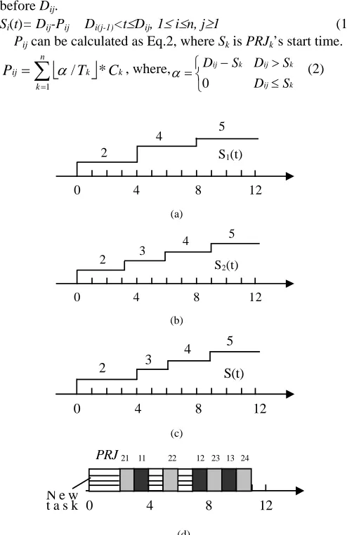
As an example, consider the two PRJs found in Fig.1 that are mapped to a single computer. Consider the case for PRJ1 where there are 4 time units before PJI11’s deadline and there are two tasks, PJI11 and PJI21, which must be completed before that time. There are therefore 2 idle time units before PJI11’s dead-line. In the case of PRJ2 there are 6 time units before PRJ22’s deadline and 3 tasks, PJI11, PJI21 and PJI22, which must be completed before that time. In this case, 3 idle time units are available before the deadline.
The above calculation can be performed for all PJIs of any
[image:4.612.51.291.507.588.2]is the sum of the execution times of PJIs that must be complete before Dij.
Si(t)= Dij-Pij Di(j-1)<t≤Dij, 1≤ i≤n, j≥1 (1) Pij can be calculated as Eq.2, where Sk is PRJk’s start time.
⎣
⎦
∑
= = n k k kij T C
P 1
* /
α
, where, (2)k ij k ij k ij S D S D S D ≤ > ⎩ ⎨ ⎧ − = 0 α
S1(t)
2
5 4
0 4 8 12
(a)
S2(t)
5
2
4 3
0 4 8 12
(b) S(t) 5 4 3 2
0 4 8 12
(c)
0 4 8 12 PRJ 21 11 22 12 23 13 24
N e w t a s k
[image:5.612.47.294.65.446.2](d)
Fig. 3. A case study of the function of idle time units (a) Function of idle time units for PRJ1 (b) Function of idle time units for PRJ2 (c) Function of idle time units for both PRJ1 and PRJ2 (d) The joint execution of PRJ1, PRJ2 and a new task with an execution time of 4 starting at 0
Fig.3.a and Fig.3.b show the functions of idle time units within a certain time period, S1(t) and S2(t), corresponding to PRJ1 and PRJ2 in Fig.1 respectively. In the figures, the time points, except zero, at which the function value increases, are called Jumping Time Points (JTP). A JTP is a PJI’s deadline. In Fig.3.a, the JTPs are 4 and 8. If the number of time units that are used to run new tasks between time 0 and any JTP are less than Si(JTP), the deadlines of all PJIs of PRJi can be guaran-teed.
Suppose n PRJs (PRJ1,..., PRJi,..., PRJn) are running on a single computer, then the distribution function of idle time left by the PRJ set, denoted as S(t), can be derived from the indi-vidual Si(t) (1≤i≤n). For any time t, S(t) obtains its value from the minimum of all Si(t), shown in Eq.3.
S(t)=min{Si(t)|1≤i≤n} (3) JTPs are also defined in S(t), as with Si(t). S(t) suggests that idle time units of S(JTP) are available in [0, JTP]. Thus, in order to satisfy the real-time requirements of all PRJs, for any
JTP, at most S(JTP) time units can be used to run new tasks in
[0, JTP]. The initial distribution of spare capabilities in each computer is constructed off-line.
S(t) corresponding to the PRJ set consisting of PRJ1 and PRJ2, is plotted in Fig. 3.c. Fig.3.d illustrates the execution of a new task in which the real-time requirements of PRJ1 and PRJ2 are still guaranteed. The execution coincides with function S(t) in Fig.3.c, that is, between time 0 and any JTP there are exactly S(JTP) time units used to run the new task.
B. On-line Modelling of the Spare Capability Distribution
If a new task starts running at any time t0, the number of idle time units in [t0, JTP] (t0<JTP), denoted by S(t0, JTP), needs to be calculated on-line. In order to do this, it is necessary to calculate the proportion of workload that all PJIs which are to complete in [0, JTP] have finished before t0, and also how much finishes in [t0, JTP]. The remaining time in [t0, JTP] will then be spare. This calculation involves identifying what PJIs must be complete before t0, and what PJIs can begin before time
t0 but must also be complete before the JTP. Some additional notation is introduced below to classify the PJIs.
PJ(t0) is a set of PJIs whose deadlines are no more than time
t0. Hence, all PJIs in PJ(t0) must be complete before t0. PJ(t0) is defined in Eq.4.
PJ(t0)={PJIij| Dij≤t0} (4)
P(t0) are denoted as the number of time units in [0, t0] that are used for running the PJIs in PJ(t0). P(t0) can be calculated using Eq.5.
⎣
⎦
∑
= = n k k k C T t P 10) / *
(
α
, where (5)k k k S t S t S t ≤ > ⎩ ⎨ ⎧ − = 0 0 0 0 α
Let JTP1, JTP2,..., JTPk be a sequence of JTPs after t0 in the spare capability distribution function S(t), and let JTP1 be the nearest to t0. LJk(t0) is a set of PJIs, whose ready times are less than t0, and whose deadlines are more than t0 but no more than
JTPk. LJk(t0) is defined in Eq.6. All PJIs in LJk(t0) can start running before t0 but must be complete before JTPk. Lk(t0) is denoted as the number of time units in [0, t0] that are used to run the PJIs in LJk(t0).
LJk(t0)={ PJIij | Rij<t0<Dij and Dij≤JTPk} (6) In Theorem 1, S(t0, JTPk) is related to S(JTPk). S(JTPk) is obtained directly from the initial spare capability distribution function established off-line in the last subsection.
Theorem 1. Suppose t0 is any time point in [0, JTPk], then
S(JTPk) and S(t0, JTPk) satisfy the following equation: S(t0, JTPk)=S(JTPk)−t0+P(t0)+Lk(t0)
(7)
Proof: PJIs whose deadlines are less than JTPk must be
com-pleted in [0, JTPk]. Their total workload is P(JTPk) (see Eq.5). The workload of P(t0) and Lk(t0) has to been finished before t0, so the workload of P(JTPk)−P(t0)− must be done in [t
)
(
t
0L
k0, JTPk]. Hence, the maximal number of time units that can be spared to run new tasks in [t0, JTPk], i.e. S(t0,JTPk), is (JTPk-t0)−(P(JTPk)−P(t0)− ). Thus, the following equation exists:
)
(
t
0L
kIn addition, JTPk−P(JTPk)=S(JTPk). Therefore Eq.7 holds. Lk(t0) in Eq.7 still remains unknown; the remainder of this subsection dedicated to this calculation.
If new tasks are run before t0, the execution of PJIs in PJ(t0) may change so that they no longer retain the original execution pattern. Theorem 2 is introduced to reveal the distribution property of the remaining time units before t0 after running the PJIs of PJ(t0) as well as any new tasks.
Theorem 2. Suppose the last executed new task is completed at
time f, then there exists some time point ts in [f, t0] (t0>f), where
1) either the PJIs in PJ(t0) retain the same execution pattern in [ts, t0] as the case when no new tasks are run before t0, or all PJIs in PJ(t0) are completed before ts, or
2) there are no idle time slots in [f, ts].
3) ts can be determined by Eq.8, where represents
the number of time units left in [t
) , ( 0 0 t t Itp s
s, t0] after executing PJIs in
PJ(t0); represents the number of time units left in
[f, t
) , ( 0 , 0 t f It A P
0] after executing both PJIs in PJ(t0) and also the new tasks. ) , ( ) ,
( 0 0, 0
0 t f I t t
Itp s = Pt A (8)
Proof: The execution of new tasks may delay the execution of
PJIs in PJ(t0). The delayed PJIs may also delay other PJIs in
PJ(t0) still further. This chain of delays will however cease when the delayed PJIs no longer delay other PJIs, or all the PJIs in PJ(t0) are complete. Since all PJIs PJ(t0) must be complete before t0, such a time point, ts, must exist that sat-isfies Theorem 2.1. Since there are unfinished workloads before ts, Theorem 2.2 also exists. Eq.8 is a direct derivation from Theorem 2.1 and 2.2. Theorem 2 is illustrated by comparing the PJIs’ execution in Fig.1.c and 3.d. In Fig.1.c, only PRJ1 and PRJ2 are run. In Fig.3.d, the current last executed new task finishes at time 7. In Fig.1.c, PJI12 and PJI23 finish at time 5 and 7 respectively. Due to the execution of the new task, PJI12 and PJI23 are delayed to finish at times 8 and 9, respectively, shown in Fig.3.d. PJI23’s delay further delays PJI13, and PJI24 is then delayed by PJI13. In Fig.3.d however, PJIs ready after time 11 can be run without further disruption. ts can be set to time 11 in the example. There are no idle time slots between time 7 and 11 (time 7 is the end-time of the new task).
As shown in Theorem 2, PJIs in PJ(t0) running in [ts, t0] re-tain the original execution pattern (as though there were no preceding new tasks). Hence the remaining time units in [ts, t0] after running these PJIs can be calculated; these time units can only be occupied by PJIs in LJk(t0). Consequently, Lk(t0) in Eq.7 can be calculated. This is shown in Algorithm 1, where IP(s, t0) is the number of time units that PJIs in LJk(t0) can occupy in time period [s, t0].
Algorithm 1. Calculating Lk(t0)
1. L←LJk(t0); Lk(t0)←0; 2. while(L≠Φ)
3. LI←the PJI with the least deadline in L; 4. c← LI’s execution time; s← LI’s ready time;
5. uf←the unfinished workload of LI; 6. if (s<ts) thens←ts;
7. if (IP(s, t0)>uf) then
8. The finished workload of LI before t0 is c; 9. Lk(t0)←Lk(t0)+c;
10. Deduct the time units used to run LI in [s, t0] from IP(ts, t0);
11. else LI’s finished workload in [0, t0]is c-uf+IP(s, t0);
Lk(t0)←Lk(t0)+c-uf+IP(s, t0);
12. Deduct the time units used to run LI in [s, t0] from IP(ts, t0);
13. L←L−LI; 14. end while
V. SCHEDULING ALGORITHMS
Let vi be a task in an ARJ. Denote stk(vi) and ftk(vi) as task vi’s earliest possible start time and its finish time on computer pk. It is assumed that tasks vi1, vi2,…, viq(viq is the last task) have been scheduled on pk. stk(vi) can be calculated using Eq.9, where, mltk(vi) is the latest time when all messages from vi’s prede-cessors arrive at pk.
otherwise rs predecesso has v v ft avt v ft v mlt v st i iq k iq k i k i k ⎪⎩ ⎪ ⎨ ⎧ = )) ( , max( )) ( ), ( max( )
( (9)
Suppose vi is scheduled on computer pk. The arrival time of the message from vi’s predecessor vj to vi (i.e. message eji) is denoted by matk(vj, vi). If vj is also scheduled on pk, then matk(vj, vi) equals ftk(vj). Suppose vj is scheduled on ps (s≠k) and there exists a message schedule sequence, ( , ),
( , ),…, ( , ), in the communication link
between p
sk
mst1 mft1sk
sk
mst2 sk
mft2 sk a
mst
sk amft
s and pk, where and are the starting time and finish time of a message transferring in the commu-nication link, respectively; then the first idle time slot in the communication link satisfying Eq.10 is used to send e
sk i
mst
mft
iskji, where comsk(eji) is the communication time of eji in the communica-tion link between ps and pk; this idle slot is (
mft
bsk,mstbsk+1).sk q
mst −max(mftqsk−1, fts(vj))≥ comsk(eji) (1≤q≤a+1, let =0, =∝) (10)
sk mft0
sk a mst +1
Thus, matk(vj, vi) can be calculated by Eq.11.
k s k s v ft e com v ft mft v v mat j k ji sk j s b i j k = ≠ ⎪⎩ ⎪ ⎨ ⎧ + = ) ( ) ( )) ( , max( ) ,
( (11)
Then, mltk(vi) in Eq.9 can be calculated by Eq.12.
mltk(vi)=max{matk(vj, vi)| vj is vi’s predecessor} (12) The complete scheduling procedure for ARJs is as follows. The global scheduler fetches an ARJ from the head of the global schedule queue, and inserts the schedulable tasks in the ARJ into the schedulable task queue. Then, at each step, the global scheduler picks a task from the head of the schedulable task queue and schedules it globally. The starting time of a task
vi is calculated as Eq.9. Suppose that vi starts at t0 on computer
t0, which can be used to run vi. Therefore, it can be determined before which JTPvi can be completed. Consequently, vi’s finish time at any computer can be determined, this is shown in Al-gorithm 2.
Algorithm 2Calculating the finish time of task vi starting at
t0 on computer pj
1. cj(cvi)← vi’s execution time on pj (predicted by PACE); 2. Calculate P(t0) using Eq.5; Get ts using Eq.8;
3. Get the first JTP after t0;
4. Call Algorithm 1 to calculate the corresponding Lk(t0); 5. Calculate S(t0, JTP) using Eq.7;
6. while (S(t0, JTP)<cj(cvi)) 7. OJTP←JTP;Get the next JTP; 8. Calculate S(t0, JTP) by Eq.7;
9. end while
10. ftj(vi)←OJTP+cj(cvi)-S(t0, OJTP);
If vi’s finish time on any computer in the cluster is greater than its deadline, the ARJ that vi belongs to is rejected. The admission control is shown in Algorithm 3.
Algorithm 3 Admission Control for task vi
1. PC←Φ;
2. for each computer pj in the cluster do
3. Calculate vi’s starting time on pj, stj(vi), using Eq.9; 4. Call Algorithm 2 to calculate vi’s finish time on pj, ftj(vi);
5. if (ftj(vi)≤dt(vi)) then 6. PC=PC∪{pj}; 7. end for
8. if PC=Φ then reject vi and the ARJ that vi belongs to; 9. else accept vi;
When vi’s deadline can be met on more than one computer, two possible Second-level Selection Policies are offered to choose a final computer. The first is a Response First (RF) policy, which selects the computer on which vi has the earliest finish time. The second is a Utilization First (UF) policy, which selects the computer on which vi has the longest execution time. The two policies are motivated in different ways. The RF pol-icy will select computers with a better performance, so that tasks can be completed sooner; the UF policy on the other hand aims to improve utilization by increasing the chance of se-lecting poorer performing computers. In section VI the per-formance of these two policies is evaluated.
After deciding which computer task vi should be scheduled to, the global scheduler resets vi’s deadline to its finish time on that computer. If all tasks in an ARJ are accepted, these tasks are then sent to the designated computers.
When the local scheduler at some computer receives the al-located ARJs’ tasks, or the PJIs of the PRJs are ready for execution, it inserts these into the Local Schedule Queue or-dered by increasing deadlines. Execution proceeds from the head of the queue and once the task with the lowest deadline is ready, the current execution is preempted.
Assuming that the initial distribution of spare capabilities on each computer in the heterogeneous cluster is constructed off-line, the on-line global dynamic scheduling algorithm
(GDS) is shown in Algorithm 4.
Algorithm 4 Global dynamic scheduling for parallel real-time jobs
1. if global scheduler queue=Φ then wait until a new ARJ arrives, then go to step 3;
2. else
3. Get a job from the head of the global scheduler queue and insert its schedulable tasks into the schedulable task queue;
4. for each task vi in the schedulable task queue do
5. Call Algorithm 3 to judge whether to accept or reject
vi;
6. if accept vithen
7. Call a second-level selection policy to choose a com-puter pj;
8. Reset vi’s deadline to be its computed finish time ftj(vi); 9. Search for new schedulable tasks in the ARJ and insert
them into the schedulable task queue; 10. else go to step 1;
11. end if
12. end for
13. Dispatch the tasks in the ARJ to the designated com-puters; go to step 1;
14.end if
Since vi’s deadline is reset to its finish time, vi will be forced to run between its starting time and the deadline. As the mod-elling analysis suggests in Section IV, vi cannot be finished earlier on the computer on which the new task is scheduled, otherwise the deadlines of some of the PJIs on that computer will be missed. In this sense, the modelling approach is optimal. When the global scheduler models the spare capacities of other computers in the cluster, no additional information has to be transferred among them to allow a scheduling decision to be made. Hence no communication overhead is incurred by the modelling approach.
VI. PERFORMANCE EVALUATION
The experimental parameters in this simulation are chosen either based on those used in the literature [12], [15] or to rep-resent a realistic workload.
Sets of 40 PRJs are randomly generated with periods ranging from 42 to 15015. The level of PRJ workloads (PLOAD) is set by varying the PRJs’ execution times. Three levels of PLOAD
(light, medium and heavy) are generated for each computer, which provides 10%, 40% and 70% system utilization, re-spectively.
In the simulation, task vi’s execution time on computer pj is calculated as ⎣cvi*pwj⎦; similarly, message eij’s communication time on link lst is ⎣mvij*lwst⎦. In a heterogeneous cluster, com-puter pi’s weight pwi is uniformly chosen between MIN_PW and MAX_PW. This range reflects the level of computational heterogeneity. The weight of a communication link is uni-formly chosen between MIN_LW and MAX_LW. This range reflects the level of communicational heterogeneity.
value of the corresponding performance measure of 10,000 independent ARJs. ARJs are assumed to arrive following a Poisson process with an arrival rate λ. Each ARJ has a ran-domly generated DAG topology with a given number of tasks (TASKNUM); task vi’s computational volume cvi is uniformly chosen between MIN_CV and MAX_CV and the volume of a message among tasks is uniformly chosen between MIN_ MV
and MAX_MV. vi’s deadline is defined as follows: if vi has no
predecessors in the DAG, dt(vi)=avt+cvi*
nw
*(dr+1), where the parameter dr is uniformly chosen between MIN_DR andMAX_DR, and
nw
is the geometric mean of the weight of all [image:8.612.338.528.120.577.2]computers; otherwise, dt(vi)=max{dt(vj)}+ cvi*
nw
*(dr+1), where vj is vi’s predecessor.TABLE I
PARAMETERS FOR SIMULATION STUDIES
Parameter Definition Value
MAX_PW/MIN_PW Maximum/minimum computer
weight 4.0/1.0 MAX_LW/MIN_LW Maximum/minimum link weight 4.0/1.0 MAX_CV/MIN_CV Maximum/minimum computation
volume 25/5
MAX_MV/MIN_MV Maximum/minimum message
volume 5/1
MAX_DR/MIN_DR Maximum/minimum deadline ratio 2.0/0
PLOAD System utilization provided by PRJs 10%, 40%, 70%
PNUM The number of computers in
a cluster 8
TASKNUM Task number in an ARJ 16
The values of the simulation parameters are given in Table 1 unless otherwise stated. Three metrics are measured in the experiments: Guarantee Ratio (GR), System Utilization (SU) and average Response Time (RT). The GR is defined as the percentage of jobs guaranteed to meet their deadlines. The SU of a cluster is defined as the fraction of time spent running tasks to the total available time in the cluster. An ARJ’s response time is defined as the difference between its arrival time and the finish time of the last task to be run. RT is the average response time for all ARJs.
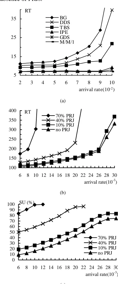
A. Job Workloads and Second-level Selection Policies
The RT can be viewed as a measure of the ability of the scheme to utilize the spare capabilities in the component computers. Fig.4.a compares the global dynamic scheduling algorithm (GDS) presented in this paper in terms of RT with four other algorithms for dynamic priority systems [5], [19], [22], [29]; i.e. Background (BG), Deadline Deferrable Server (DDS), Total Bandwidth Server (TBS) and Improved Priority Exchange (IPE). It is noted that our GDS algorithm is devised for scheduling parallel real-time jobs on a cluster, whereas the other algorithms are designed for scheduling periodic and independent aperiodic tasks (non-parallel tasks) in uniproces-sor architectures. In order to make a fair comparison, in this experiment the GDS is downgraded to schedule independent real-time tasks in a cluster of two computers, one acting as the global scheduler and the other housing a local scheduler and
jointly running tasks; the computational volumes of tasks fol-low an exponential distribution. To stress the response per-formance, GR of non-periodic real-time tasks is fixed at 1.0 by assigning extremely loose deadlines. An M/M/1 queuing model is used to compute the ideal bound for RT of the same workload in the absence of PRJs.
5 15 25 35
2 3 4 5 6 7 8 9 10
arrival rate(10-2)
RT
BG DDS T BS IPE GDS M/M/1
(a)
100 150 200 250 300 350 400
6 8 10 12 14 16 18 20 22 24 26 28 30
arrival rate(10-3) RT
70% PRJ 40% PRJ 10% PRJ no PRJ
(b)
0 10 20 30 40 50 60 70 80 90 100
6 8 10 12 14 16 18 20 22 24 26 28 30
arrival rate(10-3) SU (%)
70% PRJ 40% PRJ 10% PRJ no PRJ
(c)
Fig. 4. (a) Comparison of RT among the downgraded GDS, other traditional algorithms and an M/M/1 queuing model; PLOAD=40%, the average compu-tational volume of tasks is 8 and the computer weight is 1.0 (b) Comparison between the GDS and the ideal bound (no PRJ); MAX_CV/MIN_CV=12/4, RF policy (c) The corresponding SU for the workloads in Fig.4.b
[image:8.612.47.297.240.393.2]cluster of 8 computers under different levels of PLOAD. An ideal bound of RT is generated for comparison by running the same ARJ workloads in the same heterogeneous cluster in the absence of any PRJs. The GR of the ARJs is also fixed to be 1.0. It is observed from Fig.4.b that in the case of 10% PLOAD, the RT obtained by the GDS scheme is very close to the ideal bound, indicating the excellent performance of GDS in utiliz-ing spare capabilities in the schedulutiliz-ing of parallel real-time jobs on a cluster. We also observe that in the case of 40% or 70% PLOAD, RT increases dramatically once λ is greater than
some critical value. This is because the system utilization reaches a maximum value at that arrival rate. At 70% PLOAD, the maximum system utilization is near 100%, while at 40% the maximum is 97% (under the workload parameters selected for this experiment), this is shown in Fig.4.c. It is also observed from Fig.4.c that the maximum system utilization that can be reached under pure ARJ workloads is about 75%. The reason that the maximum system utilization is less than 100% is simply because of the existence of message passing and precedence constraints among the tasks in the ARJs.
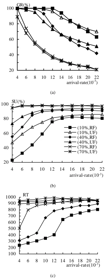
As stated in Section V, when the deadline of a task in an ARJ can be met on more than one computer, the Response First (RF) policy or Utilization First (UF) policy are offered to aid the final selection. Fig.5.a, b and c display the metrics GR, SU and RT as the function of λ under these two policies, respectively. The first observation from Fig.5.a is that GR decreases as λ increases in all cases, as expected. A further observation is that in the case of 10% and 40% PLOAD, the RF policy outper-forms UF when λ is low, whereas when λ exceeds a certain threshold the opposite is true. This is explained as follows. The RF policy is predisposed to choosing the better computers, whereas the UF policy has the opposite trait. When the ARJ workload is light, that is, not all computers are busy, allocating tasks to better computers will mean that there is more chance that the whole ARJ is accepted. By increasing the value of λ, we simulate all computers receiving new heavy workloads under both policies. In this context, under the UF policy and when tasks cannot be assigned to poorer computers, they have a greater chance of being allocated to better computers in order to meet their deadlines, compared with that of the RF policy which has the opposite selection preference. The experimental results suggest that when the ARJ workload is so high that all the computers in a heterogeneous cluster are heavily occupied, allocating workload to poorer nodes as opposed to better nodes is highly desirable.
As can be observed from Fig.5.b, SU increases as λ in-creases, as is to be expected. It is also observed that the UF policy outperforms the RF policy in terms of SU in cases of 10% and 40% PLOAD, especially when λ is low. This is
be-cause allocating a task to a poorer computer will lead to a greater increase in SU, if the makespan of the new task work-load in the cluster remain unchanged (or increase by some small percentage). If the allocation of a task incurs a large increase in makespan however, the allocation may decrease the SU. Fortunately, such an allocation has less chance of passing
the admission control since it implies a very late finish for the task. Hence, through the filtering function provided by the admission control, the UF policy contributes more to the im-provement of SU than does the RF policy. The experimental results suggest that utilization of the cluster is significantly enhanced compared with the original PLOAD.
20 40 60 80 100
4 6 8 10 12 14 16 18 20 22
arrival-rate(10-3) GR(%)
(a)
20 40 60 80 100
4 6 8 10 12 14 16 18 20 22
arrival-rate(10-3)
SU(%)
(10%,RF) (10%,UF) (40%,RF) (40%,UF) (70%,RF) (70%,UF)
(b)
100 200 300 400 500 600 700 800 900 1000
4 6 8 10 12 14 16 18 20 22
arrival-rate(10-3)
RT
[image:9.612.348.531.127.605.2](c)
Fig. 5. Effect of Job workloads and second-level selection policy on (a) GR (b) SU and (c) RT, Legends for Fig.5.a and c are the same as those in Fig.5.b
PLOAD in the cluster is high, there are a limited number of computers that satisfy the admission control.
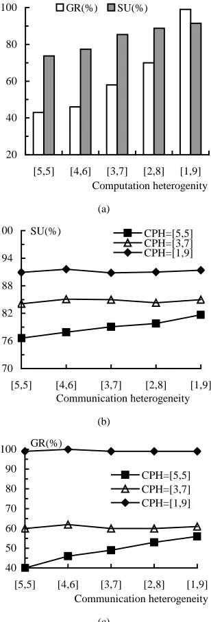
[image:10.612.97.251.175.629.2]B. Computation and Communication Heterogeneity
Fig.6.a shows the impact of computation heterogeneity on the metrics GR and SU. Fig.6.b and Fig.6.c show the impact of
communication heterogeneity on GR and SU, respectively, under different levels of computation heterogeneity. Only the results for 40% PLOAD and the RF policy are shown, the re-sults for the other cases demonstrate similar behaviour.
20 40 60 80 100
[5,5] [4,6] [3,7] [2,8] [1,9]
Computation heterogenity
GR(%) SU(%)
(a)
70 76 82 88 94 100
[5,5] [4,6] [3,7] [2,8] [1,9]
Communication heterogeneity
SU(%) CPH=[5,5]
CPH=[3,7] CPH=[1,9]
(b)
40 50 60 70 80 90 100
[5,5] [4,6] [3,7] [2,8] [1,9]
Communication heterogeneity GR(%)
CPH=[5,5] CPH=[3,7] CPH=[1,9]
(c)
Fig. 6. Effect of computation and communication heterogeneity, the RF policy and PLOAD=40% (a) Effect of computation heterogeneity on GR and SU,
λ=0.006 (b) Effect of the communication heterogeneity on SU, λ=0.006 (c) Effect of the communication heterogeneity on GR, λ=0.006
The levels of computation and communication heterogeneity are measured by the scale of the range from which computer weights and communication link weights are selected. Five sets of computer and link weights, all with the same average, are
uniformly chosen from five ranges, [1,9], [2,8], [3,7], [4,6] and [5,5].
As can be observed from Fig.6.a, GR and SU improve as the computation heterogeneity increases. The increase in GR may be because as the computation heterogeneity increases, the increasing variance in a task’s execution time provides the task with more chance of fitting into the idle time slots before its deadline. Under the same workload, the increase in GR leads to an increase in SU. It can be observed from Fig.6.b and Fig.6.c that SU and GR increase as the communication heterogeneity increases in the case when the computation heterogeneity is [5,5] (i.e. homogeneity). This may be because the increasing variance in message transfer time provides more chance of finding a suitable idle time slot in the communication channels. However, the communication heterogeneity has no obvious impact on SU and GR when the computation heterogeneity increases to [3,7] or [1,9]. This suggests that the level of computation heterogeneity is more critical for scheduling ARJs than the level of communication heterogeneity. The results suggest that the performance of the constituent computers in the cluster should be carefully selected so as to achieve bal-anced system performance.
C. Task Size and Message Size
Fig.7.a shows the impact of the size of tasks in ARJs on GR and SU. Only the results for 40% PLOAD are shown as the results for other levels of PLOAD display similar behaviour. The task size is measured by the average computational volume of tasks in an ARJ. In this experiment, when the task size in-creases, the average arrival rate λ is set to decrease propor-tionally so as to keep the total ARJ workload unchanged.
As can be observed from Fig.7.a, under the RF policy the impact of the task size is mixed. On the one hand, GR retains 100% and then decreases as the task size increases. This is because the longer a task is run, the more chance there is that the task is disrupted by the PRJs. It can be concluded from this result that under the same workload this admission control will favour dense, short new jobs. On the other hand, SU improves as the task size increases. This is because under the RF policy, a lower GR may imply that a large number of tasks are being allocated to poorer computers, which contributes to an im-provement in SU. Under the UF policy, GR decreases, but SU remains stable as the task size increases. This may be because the UF policy allocates tasks to poorer computers, so the de-cline in GR has no obvious impact on SU.
Fig.7.b and Fig.7.c demonstrate the effect of the ratio of the task size to the size of messages among tasks on GR, SU and RT. Again, only the results for 40% PLOAD and the RF policy are presented. The message size of an ARJ is measured by the average volume of all messages among the tasks in the ARJ. The task-size/message-size ratio varies from 15/3 to 3/15, all with the same volume sum. As can be observed from Fig.7.b, The impact of the task-size/message-size ratio is also mixed. The GR improves whereas the SU decreases as the
ad-mitted as demonstrated above; second, although the message size increases as the Task-size/message-size ratio decreases, the scheduling policy may compensate for this by scheduling two tasks on the same computer if the communication time between them is too large; and finally, computers are shared by ARJs and PRJs, while the communication links are exclusively util-ized by ARJs. Fig.7.c shows that the RT decreases as the
Task-size/message-size ratio decreases. These results suggest that the task size is more critical than the message size when guaranteeing the ARJ’s admission and response time.
60 70 80 90 100
5 10 15 20 25 30
Task size
(GR,RF) (SU,RF)
(GR,UF) (SU,UF)
(a)
20 40 60 80 100
15/3 12/6 9/9 6/12 3/15
Task size/Message size
GR(%) SU(%)
(b)
0 100 200 300 400 500 600 700 800
15/3 12/6 9/9 6/12 3/15
Task size/Message size RT
[image:11.612.93.260.176.661.2](c)
Fig. 7. Effect of task and message size, PLOAD=40% (a) Effect of task size on
GR and SU, λ is 0.025 when the task size is 5 (b) Effect of
task-size/message-size ratio on GR and SU, λ=0.02, RF (c) Effect of task-size/message-size ratio on RT, with the same parameters as those in Fig.7.b
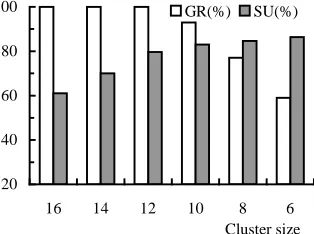
D. Cluster Size
The cluster size is changed in such a way as to keep the PRJ
and PLJ workload unchanged while gradually removing the poorer computers from the cluster. As can be observed from Fig.8, the GR retains 100% when the number of computers in the cluster decreases from 16 to 12, and decreases when the cluster size decreases further from 12 to 6, while the SU im-proves as the cluster size decreases, as expected. Fig.8 suggests that a cluster with more than 12 computers is inefficient. This result indicates that the cluster size should be carefully selected based on experimental evidence so that a good cost-performance ratio can be achieved.
20 40 60 80 100
16 14 12 10 8 6
Cluster size
[image:11.612.363.520.181.298.2]GR(%) SU(%)
Fig. 8. Effect of the cluster size on GR and SU, λ=0.02, PLOAD is 10% in each computer as the number of computers is 16
VII. CONCLUSIONS
This paper presents a scheduling framework for dynamic aperiodic parallel real time jobs, which is based on modelling the spare capabilities of a heterogeneous cluster on which pe-riodic real-time jobs are running. The approach used in mod-elling spare capabilities is optimal in the sense that once a new task starts running, it will utilize all the spare capabilities and its finish time is the earliest possible. No communication over-heads are incurred by this approach. Scheduling ARJs takes both task and message scheduling into account. Extensive simulations have been conducted that demonstrate that system utilization is significantly enhanced without impacting on the QoS of existing jobs. Future work is planed to extend this scheduling framework to include additional prediction, sched-uling and dispatch times.
REFERENCES
[1] M. Apte, S. Chakravarthi, J. Padmanabhan and A. Skiellum, “A syn-chronized real-time linux based Myrinet cluster for deterministic high performance computing and MPI/RT,” 15th International Parallel and Distributed Processing Symposium, 2001.
[2] T.F. Abdelzaher, K.G. Shin,“Combined task and message scheduling in distributed real-time systems,” IEEE Transactions on parallel and dis-tributed systems, 10(11), November 1999.
[3] H. Aydin, R. Melhem, D. Mosse, and P. Mejia-Alvarez, “Optimal re-ward-based scheduling of periodic real-time tasks,” 20th IEEE Real-Time Systems Symposium, December 1999.
[4] M.A. Bonuccelli, M. C Clò, “EDD algorithm performance guarantee for periodic hard-real-time scheduling in distributed systems,” 15th Interna-tional Parallel and Distributed Processing Symposium, 1999.
[5] M. Caccamo, G. Lipari, and G. Buttazzo, “Sharing resources with the TB* server,” IEEE Real-Time Systems Symposium, 1999.
[7] D.B. Golub, “Operating system support for coexistence of real-time and conventional scheduling,” The 1st Symposium on Operating Systems Design and Implementation, 1994.
[8] L. He, H. Jin, Y. Chen and Z. Han, “Optimal scheduling of aperiodic jobs on cluster system,” 7th International Conference on Parallel and Dis-tributed Computing (Euro-Par 2001), Manchester, UK, 2001, pp.764-772. [9] K. Hwang and Z. Xu, Scalable Parallel Computing: Technology,
Archi-tecture, Programming. McGraw Hill, 1998.
[10] D. Kebbal, E.G. Talbi, J.M. Geib, “Building and scheduling parallel adaptive applications in heterogeneous environments,” 1st IEEE Com-puter Society International Workshop on Cluster Computing, December, 1999.
[11] Y. Kwok, “Parallel program execution on a heterogeneous PC cluster using Task Duplication,” 9th Heterogeneous Computing Workshop, 2000.
[12] J. P. Lehoczky and S. Ramos-Thuel, “An optimal algorithm for schedul-ing soft-aperiodic tasks in fixed-priority preemptive systems,” Proc. of Real-Time Systems Symposium, 1992, pp.110-123.
[13] C.W. Mercer, S. Savage, and H. Tokuda, “Processor capacity reserves: operating system support for multimedia applications,” Proc. of the IEEE International Conference on Multimedia Computing and Systems, 1994. [14] G.R. Nudd, D.J. Kerbyson et al, “PACE-a toolset for the performance
prediction of parallel and distributed systems,” Intl Journal of High Performance Computing Applications, Special Issue on Performance Modelling, 14(3), 2000, 228-251.
[15] X. Qin and H. Jiang, “Dynamic, reliability-driven scheduling of parallel real-time jobs in heterogeneous systems,” 30th International Conference on Parallel Processing, Valencia, Spain, September 3-7, 2001. [16] A. Radulescu, A. Gemund, “A low-cost approach towards mixed task and
data parallel scheduling,” International Conference on Parallel Proc-essing, 2001.
[17] S. Ranaweera, and D.P. Agrawal, “Scheduling of periodic time critical applications for pipelined execution on heterogeneous systems,” Proc. of the 2001 International Conference on Parallel Processing, 2001. [18] S. Ranaweera, D.P. Agrawal, “Task duplication based scheduling
algo-rithm for heterogeneous systems,” International Parallel and Distributed Processing Symposium, 2000.
[19] D.A.E. Salaheddine, “Aperiodic scheduling in a dynamic real-time manufacturing system,” IEEE Real-Time Embedded System Workshop, 2001.
[20] S. Sinha and M. Parashar, “Adaptive runtime partitioning of AMR ap-plications on heterogeneous clusters,” 3rd IEEE Intl Conf on Cluster Computing, 2001.
[21] D.P. Spooner, S.A. Jarvis, J. Cao, S. Saini and GR. Nudd, “Local grid scheduling techniques using performance prediction,” IEE
Proc-Computers and Digital Techniques, 150(2): 87-96, 2003. [22] M. Spuri and G. Buttazzo, “Scheduling aperiodic tasks in dynamic
prior-ity systems,” Real-Time Systems, 10(2), 1996, 179-210.
[23] B. Srinivasan, S. Pather, F. Ansari, and D. Niehaus, “A firm real-time system implementation using commercial off-the-shelf hardware and free software,” 4th IEEE Real-Time Technology and Applications Symposium, 1998
[24] M. Suzuki, H. Kobayashi, N. Yamasaki, and Y. Anzai, “A task migration scheme for high performance real-time cluster system,” 19th Interna-tional Conference on Computers and Their Applications, pp. 228-231, 2003
[25] X.Y. Tang, S.T. Chanson, “Optimizing static job scheduling in a network of heterogeneous computers,” 29th Intl Conference on Parallel Proc-essing, 2000.
[26] K. Taura, A. Chien, “A heuristic algorithm for mapping communicating tasks on heterogeneous resources,” 9th Heterogeneous Computing Workshop, 2000.
[27] M. Thomadakis and J. Liu, “On the efficient scheduling of non-periodic tasks in hard real-time systems,” IEEE Real-time System Symposium, 1999.
[28] H. Topcuoglu, S. Hariri and M. Wu, “Task scheduling algorithms for heterogeneous processors,” 8th Heterogeneous Computing Workshop, 1999.
[29] S. Wang, Y.C. Wang, K. Lin,“Integrating the fixed priority scheduling and the total bandwidth server for aperiodic tasks,” 7th International Conference on Real-Time Systems and Applications, 2000.
[30] M. Wu, W. Shu and Y. Chen, “Runtime parallel incremental scheduling of DAGs,” International Conference on Parallel Processing, 2000.
Ligang He is a PhD student and research associate in the High Performance System Group in the Department of Computer Science at the University of Warwick, United Kingdom. His areas of interests are cluster computing, grid computing, real-time scheduling and performance prediction. He is a student member of the IEEE.
Dr. Stephen Jarvis is a Senior Lecturer in the High Performance System Group at the University of Warwick. He has authored over 50 referred publications (including three books) in the area of software and performance evaluation. While previously at the Oxford University Computing Laboratory, he worked on performance tools for a number of different programming paradigms in-cluding the Bulk Synchronous Parallel (BSP) programming library – with Oxford Parallel and Sychron Ltd – and the Glasgow Haskell Compiler – with Glasgow University and Microsoft Research in Cambridge. He has close research links with IBM, including current projects with IBM’s TJ Watson Research Center in New York and with their development centre at Hursley Park in the UK. Dr Jarvis sits on a number of international programme com-mittees for high-performance computing, autonomic computing and active middleware; he is also the Manager of the Midlands e-Science Technical Forum on Grid Technologies.
Daniel Spooner is a newly-appointed Lecturer in the Department of Computer Science and is a member of the High Performance System Group. He has 15 referred publications on the generation and application of analytical perform-ance models to Grid computing systems. He has collaborated with NASA on the development of performance-aware schedulers and has extended these through the e-Science Programme for multi-domain resource management. He has worked at the Performance and Architectures Laboratory at the Los Alamos National Laboratory on performance tools development for ASCI applications and architectures.