Economic forecasting in a changing world

University of Warwick institutional repository: http://go.warwick.ac.uk/wrap This paper is made available online in accordance with

publisher policies. Please scroll down to view the document itself. Please refer to the repository record for this item and our policy information available from the repository home page for further information.

To see the final version of this paper please visit the publisher’s website. Access to the published version may require a subscription.

Author(s): Michael P. Clements and David F. Hendry Article Title: Economic Forecasting in a Changing World Year of publication: 2008

Capitalism and Society

Volume3,Issue2 2008 Article1

Economic Forecasting in a Changing World

Michael P. Clements

David F. Hendry

∗_{University of Warwick, M.P.Clements@warwick.ac.uk}

†_{Oxford University, DAVID.HENDRY@NUFFIELD.OX.AC.UK}

Economic Forecasting in a Changing World

Michael P. Clements and David F. Hendry

Abstract

This article explains the basis for a theory of economic forecasting developed over the past decade by the authors. The research has resulted in numerous articles in academic journals, two monographs, Forecasting Economic Time Series, 1998, Cambridge University Press, and Fore-casting Nonstationary Economic Time Series, 1999, MIT Press, and three edited volumes, Under-standing Economic Forecasts, 2001, MIT Press, A Companion to Economic Forecasting, 2002, Blackwells, and theOxford Bulletin of Economics and Statistics, 2005. The aim here is to provide an accessible, non-technical, account of the main ideas. The interested reader is referred to the monographs for derivations, simulation evidence, and further empirical illustrations, which in turn reference the original articles and related material, and provide bibliographic perspective.

∗_{The background research has been generously financed by the United Kingdom Economic and}

1

Introduction

The main challenge facing any theory of economic forecasting is to explain the re-current episodes of systematic mis-forecasting that have occurred historically, there-by helping to develop methods which avoid repeating such mistakes in the future. UK examples of serious forecast failure include: missing the stagflation of the 1970s, the consumer boom of the mid 1980s, and the depth of the recession in the early 1990s. Other examples also abound, and include the collapse in South-East Asia– Barrell (2001) notes six major episodes of change during the 1990s alone. It is perhaps unsurprising that changed economic circumstances in response to dramatic oil price rises, financial deregulation, and so on, are an important ingredient in ex-plaining forecast failure, but less obviously, from the theory discussed below we are able to deduce: what types of changes in economic behavior are most deleterious for the popular classes of economic forecasting models; what can be done to improve the performance of such models in the face of structural breaks; and what factors and mistakes do not usually cause forecast failure. This article explains the basis for such deductions.

Economies evolve over time and are subject to intermittent, and sometimes large, unanticipated shifts. Such breaks may be precipitated by changes in legislation, sudden switches in economic policy, major discoveries and innovations, or political turmoil. Examples relevant to the UK include the abolition of exchange controls, the introduction of interest-bearing checking accounts, membership of the Euro-pean Union, privatization, and wars. The models used to understand and forecast processes as complicated as large national economies are far from perfect represen-tations of their behavior. Moreover, the data series used in model building are often inaccurate, prone to revision, and may be provided only after a non-negligible delay. Usually, forecasters are only dimly aware of what changes are afoot, and even when developments can be envisaged, may find it hard to quantify their likely impacts (e.g., the effects of financial deregulation on UK consumers’ spending in the late 1980s). Thus, to understand the properties of economic forecasts, a viable theory must allow for a complicated, high dimensional economy which:

(a) unexpectedly shifts at unanticipated times;

(b) is measured by inaccurate, limited and changing data;

(c) is forecast by models which are incorrectly specified in unknown ways.

Such a theory reveals that many of the conclusions that can be established for-mally for correctly-specified forecasting models of constant-parameter economies no longer hold. For example, since the distributions of future outcomes are not the same as those in-sample, it cannot be established that the current conditional expec-tation is the minimum mean-square forecasting device; that well-specified models will forecast better than badly specified; that causally-relevant variables will forecast better than irrelevant ones; and that further ahead interval forecasts must be larger than near-horizon ones. Such implications may seem highly damaging to the fore-casting enterprise, and indeed are for some ‘conventional’ approaches, but they are far from precluding useful forecasts.

Instead, our theory gives rise to a very different set of predictions about the properties of existing forecasting tools–most importantly that shifts in the means of variables (location shifts) are the most pernicious change for forecasting mod-els, and there are all too many location shifts in economic time series. Forecasting devices that are robust in the face of location shifts will not experience systematic forecast failure; these are the class that should dominate in forecasting competitions (such as Makridakis and Hibon, 2000); whereas the poor historical track record of econometric systems–often out-performed by ‘naive devices’–which dates from the early history of econometrics, is due to location shifts. We have evaluated these implications both in specific empirical settings and using computer simulations, and obtained a fairly close concordance between theory and evidence. The findings con-firm that despite its non-specific assumptions, a theory of forecasting which allows for unanticipated structural breaks in an evolving economic mechanism for which the econometric model is mis-specified in unknown ways, can nevertheless provide a useful basis for interpreting, and potentially circumventing, systematic forecast failure in economics.

Forecast failure is formally defined as forecasts being significantly less accurate than expected given how well the model explains the data over the past, or com-pared to an earlier forecast record. This is a distinct concept from that of ‘poor’ forecasts, where forecasts may be judged as being poor relative to the forecasts of a rival model, or relative to some standard set in light of the requirements for which the forecasts are to be used. Forecasts are increasingly judged by their value for decision-makers (see Pesaran and Skouras, 2002, for a recent review), whereas comparison against rival forecasts is often performed using tests of equal forecast accuracy (see, e.g., West, 2006) or tests of forecast encompassing (e.g., Clements and Harvey, 2008). Forecasts may be poor simply because a series is inherently volatile, and this is not the same as forecast failure, the phenomenon we are primar-ily interested in explaining. When forecasts from a particular model or forecasting method are sometimes significantly worse than from a rival approach, the possibility arises that a combination of the two sets of forecasts may be beneficial.

2 http://www.bepress.com/cas/vol3/iss2/art1

An important distinction is between ex-ante forecast failure and ex-post predic-tive failure. Ex ante failure relates to incorrect statements about as yet unobserved events, and could be due to many causes, including data measurement errors or false assumptions about non-modeled variables which are corrected later, so the forecast-ing model remains constant when updated. Thus, ex-ante forecast failure is primarily a function of forecast-period events. Ex-post predictive failure entails rejection of a model against the observed outcomes by a valid parameter-constancy test, and oc-curs when a model is non-constant on the whole available information set, and is a well-established notion.

2

Outline

The plan of the remainder of this exposition is as follows. Section 3 analyses fore-casting models, distinguishing between error correction and equilibrium correction. Somewhat paradoxically, models formerly known as ‘error-correction models’ (see e.g. Davidson, Hendry, Srba and Yeo, 1978) do not in fact ‘error correct’ when equilibria shift, so are actually equilibrium-correction models (EqCMs). A prob-lem with such models is that when the equilibrium shifts, EqCMs still converge to their in-built equilibria. Consequently, this class of model is prone to systematic failure. Shifts in equilibrium means are the most important example of location shifts. Conversely, models with an additional imposed unit root, irrespective of the process being modeled having a stochastic trend or not, do error correct to loca-tion shifts. This distincloca-tion is at the heart of understanding why, say, the random-walk and the Box–Jenkins time-series method, can prove hard to beat. The class of EqCMs is huge and includes most widely-used forecasting models, such as regres-sions, dynamic systems, vector autoregressions (VARs), dynamic-stochastic general equilibrium models (DSGEs), vector equilibrium-correction models (VEqCMs: see e.g., Hendry and Juselius, 2000, 2001), autoregressive conditional heteroskedastic (ARCH) processes, and generalized ARCH (GARCH: see Engle, 1982, and Boller-slev, 1986), as well as some other volatility models. Thus, the failure of EqCMs to adjust to equilibrium shifts has far-reaching implications. Although the majority of the macroeconomic forecasting literature is concerned with forecasting the cen-tral tendency or conditional first moment of the variable of interest, there is also much interest in forecasting the volatility of financial time series, such as returns on assets, that is, forecasting the conditional variance of such series. As the reference above to GARCH models as members of the EqCM class suggests, the problems that afflict first-moment forecasts are also relevant for equilibrium-correcting volatility forecasting models (see Clements and Hendry, 2006, p.614-7).

distribution. Section 3.3 considers a number of factors traditionally assigned a major role in forecast failure, but which, in the absence of parameter non-constancies, would appear to play only a minor role. Section 4 discusses how to tackle forecast failure: section 4.1 illustrates with the empirical example of forecasting UK M1, and sections 4.2, 4.3 and 4.4 discuss methods that might help circumvent forecast failure once a potentially damaging change in economic conditions has occurred. Finally, section 5 briefly considers some implications of our theory of economic forecasting.

3

Forecasting models

Econometric forecasting models comprise systems of relationships between vari-ables of interest (such as GNP, inflation, exchange rates etc.), where the relation-ships are estimated from available data, usually aggregate time series. The equa-tions in such models have three main components: deterministic terms (such as in-tercepts and linear trends) that capture the levels and trends, and whose future values are known; observed stochastic variables (like consumers’ expenditure, prices, etc.) with unknown future values, which are also the target of forecasting; and unobserved errors, all of whose values (past, present and future) are unknown, though perhaps estimable in the context of a given model. The relationships between these compo-nents could be inappropriately formulated in the model, inaccurately estimated, or could change in unanticipated ways. This leads to nine types of mistake, any or all of which could induce poor forecast performance, either from inaccurate (i.e., biased), or imprecise (i.e., high variance) forecasts. Instead, we find that some mistakes have pernicious effects on forecasts, whereas others are relatively less important in most settings. Moreover, ‘correcting’ one form of mistake may yield no improvement in forecast accuracy when other mistakes remain. For example, more sophisticated methods for estimating unknown parameters will not help when the problem is an unanticipated trend shift.

In a world plagued by non-constancies, it cannot be demonstrated that effort devoted to model specification and estimation will yield positive returns to

forecast-ing—‘good models, well estimated, and well tested’ will not necessarily forecast

better than ‘poor’ ones (in the sense of models which are not well fitting, or fail residual diagnostic tests, etc.). The degrees of congruence or non-congruence of a model with economic theory and data transpire to be neither necessary nor sufficient for forecasting success or failure. However, our forecasting theory clarifies why such a result holds, and why it is not antithetical to developing congruent economet-ric models for other purposes such as testing theories, understanding the economy, or conducting economic policy. Indeed, different ways of using the same models are required for forecasting and policy. Moreover, our theory suggests methods by

4 http://www.bepress.com/cas/vol3/iss2/art1

which existing econometric models can be made more robust to non-constancies, some of which are already in use but have previously lacked rigorous analysis of their properties. It has long been known that a given model can produce very differ-ent forecasts depending on how it is ‘adjusted’, for example, by intercept corrections that set the model ‘back on track at the forecast origin’. Such a result immediately reveals why the forecast records of models may not be closely related to their empir-ical verisimilitudes: the corrections alone may determine the success or otherwise of the forecasts. However, a sequence of accurate policy predictions requires that the economy behaves in a similar manner to the model, so does entail a high-quality model.

Most econometric systems now embody cointegrated relations driven by sto-chastic trends. Cointegration has helped formalize the concept of steady-state equi-libria in non-stationary processes, and has been the subject of a Nobel Prize award to Sir Clive Granger (see Hendry, 2004). Even in evolving economies, equilibrium means exist which determine the values towards which an economy would adjust in the absence of further ‘shocks’: possible examples include the savings rate, the real rate of interest, the long-run growth rate, and the velocity of circulation. Eco-nomic equilibria usually involve combinations of variables, as with all the examples just cited. Nevertheless, in a forecasting context, cointegration can be a double-edged sword. On the one hand, by tying together series that are indeed linked in the long-run, forecasts thereof do not drift apart, improving both forecast accuracy and understanding. On the other hand, our research shows that the treatment of equi-librium means in forecasting models is about the most crucial factor in determining forecasting performance. The key to understanding systematic forecast failure, and its avoidance, turns on four aspects of such equilibrium means.

First, their specification and estimation: inadequate representations or inaccurate estimates of equilibrium means can induce poor forecasts.

Secondly, the consequences of unanticipated changes in their values are espe-cially pernicious: the economy converges to its new equilibrium means, but the forecasting model remains at the old values inducing a systematic divergence.

Thirdly, successfully modeling movements in equilibrium means can pay hand-some dividends, even if only by using corrections and updates to offset changes.

Finally, formulating models to minimize the impact of changes in equilibrium means is generally beneficial, even when the cost is a poorer representation of both the economic theory and the data. Various strategies can be adopted which help at-tenuate the impacts of shifts in equilibrium means, including intercept corrections, over-differencing, co-breaking, and modeling regime switches.

−4 −3 −2 −1 0 1 2 3 4 5 6 7 8 9 10 0.05

0.10 0.15 0.20 0.25 0.30 0.35 0.40

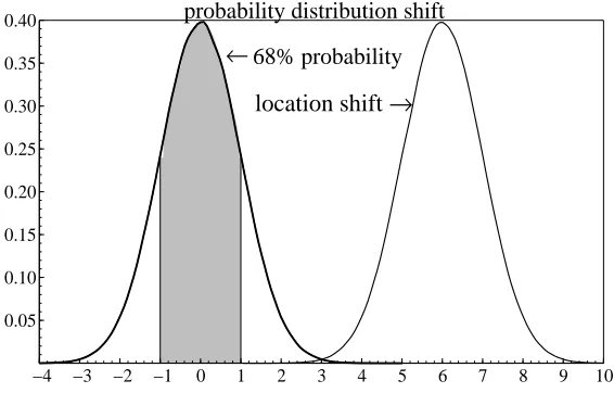
location shift →

probability distribution shift

68% probability

←

Figure 1: Location shift in a probability distribution

outcome between ±1with 68% probability, with low probabilities attached to out-comes outside±2. After the shift, there is an almost zero probability of observing an outcome within_±2. The ex ante conditional expectation is zero, and ex post, that is a very poor forecast.

If the shift was impossible to anticipate, little can be done to mitigate the imme-diate forecast error. The key is what happens in the next period, both to the shift and to the forecasting model. Many shifts seem highly persistent after their occur-rence, so retaining the original model unchanged is rarely a good strategy. Of course, the shift could be temporary, for example, simply a measurement error which will be corrected in the next period. However, systematic forecast failure is sufficiently common to suggest that many shifts are not measurement artifacts and are persistent, so the model needs to adapt rapidly to the changed environment if persistent errors are to be avoided. We return to this issue below.

The economic environment may change so that relationships between variables embodied in the model no longer hold, or changes may result indirectly from changes in the economic mechanism which are not explicitly represented in the model. Of all the possible sorts of changes, it is those which induce a mismatch between the means of the data and the model predictions that are most problematic. Relative to the role played by location shifts, other forms of mis-specification seem to have a less pernicious effect on forecast accuracy. Indeed, the next most important cause of forecast failure, after shifts in deterministic factors over the forecast horizon, is mis-specification of deterministic terms. For example, omitting a trend in a model when there is one in the data rapidly leads to large forecast errors, resulting from a mismatch between the model and data means.

6 http://www.bepress.com/cas/vol3/iss2/art1

3.1

Shifts versus fat tails

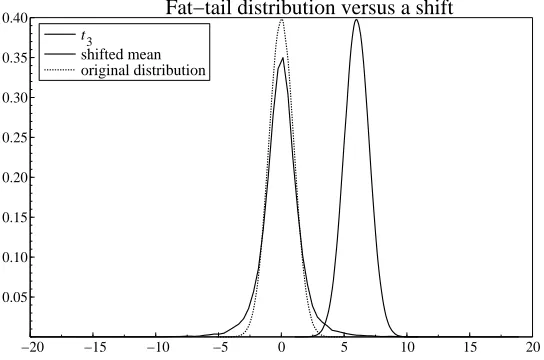
In financial data analysis, it is common to allow for distributions with fatter tails than the normal, to take account of ‘outliers’. Figure 2 compares that approach with the location-shift interpretation, using at_{3-distribution, which has only its first}

two moments finite. There are major differences between the two representations of the sudden change. First,t_{3 covers a huge range with non-zero, albeit very small,}

probability, whereas the ex post range has not changed in the location shift distribu-tion, and although it certainly could, that would not alter the impact. Second, there remains a very small probability when the fat-tailed distribution is correct of observ-ing the shifted mean outcome, and even smaller probabilities for values above its mean. Third, the next draw from the two distributions will occur with very different probabilities–the fat tail could easily be a negative value, whereas the location shift has essentially no probability of such an outcome.

−20 −15 −10 −5 0 5 10 15 20

0.05 0.10 0.15 0.20 0.25 0.30 0.35

0.40 Fat−tail distribution versus a shift

t₃

shifted mean original distribution

Figure 2: Location shift versus a fat-tailed distribution

Financial models also allow for dependence between shocks, as in ARCH or GARCH models, so that a large draw in one period induces a large shock in the next period–but again of either sign. This correctly reflects increased volatility, not a location shift.

3.2

Persistence of shifts

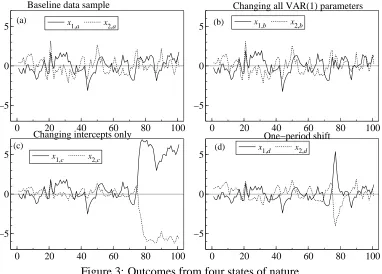
depends on the last period’s values of both variables, typical of models used to de-scribe economic data. In the figure:

(a) is the baseline, with no parameter changes;

(b) is when all intercept and dynamic feedback parameters are shifted dramatically, by between 30 and 100 error standard deviations, but maintaining the same equilib-rium means for the remainder of the sample after the break;

(c) records when only the equilibrium means are altered, in this case, by just three error standard deviations, again for the remainder of the sample; and

(d) reports the outcomes when the equilibrium means are again shifted by just three error standard deviations, but for one period only, and then revert back to their pre-break values.

0 20 40 60 80 100

−5 0 5

Baseline data sample

(a) x_1,a x_2,a

0 20 40 60 80 100

−5 0 5

Changing all VAR(1) parameters

(b) x_1,b x_2,b

0 20 40 60 80 100

−5 0 5

Changing intercepts only

(c)

x_1,c x_2,c

0 20 40 60 80 100

−5 0 5

One−period shift

(d) x_1,d x_2,d

Figure 3: Outcomes from four states of nature

As can be seen, (a) and (b) are almost identical despite the enormity of the shifts in the VAR in (b), yet the existence of this surprising phenomenon was deduced directly from our theoretical analysis, as were the drastic changes visible in (c) and (d) despite the much smaller sizes of their shifts, with that in (d) even being for just one observation.

Thus, location shifts have pernicious effects, can explain forecast failure, and differ substantively from fat-tailed distributions even with GARCH persistence. The obvious question is then–but is that the correct explanation? To resolve that, we first

8 http://www.bepress.com/cas/vol3/iss2/art1

need to exclude other possible explanations and then to establish that economic time series show characteristics like figure 3(c). We address those points in turn.

3.3

Other sources of forecast errors

There are, of course, many sources of forecast error besides location shifts. These include the model being mis-specified, in the sense that relevant variables that in reality affect the variable being forecast are omitted, or extraneous variables are in-cluded, or the way in which the various influences interact together is incorrect, etc. All of these might be thought to bear on the properties of the forecasts obtained from the model. Another source arises from the effects of the different influences being imprecisely estimated from the data. We may believe we know what the important factors to be included are, but not know the magnitudes of these individual factors. These have to be learnt from estimating the model on past data, yet there may be in-sufficient information in the data to pin down these effects with any precision. This imprecision is usually termed parameter estimation uncertainty, and will depend in part on the magnitude of the ‘shocks’ over the historical period. These sources of forecast error do matter, but are less important than location shifts, except in so far as they concern deterministic terms. For example, an inaccurately-estimated linear trend can also induce serious forecast errors. To draw on an analogy from Kuhn (1962), all these aspects may matter in ‘normal forecasting’, and contribute to a worse forecasting performance than would prevail in their absence (e.g., with a correctly-specified model and known parameter values), but location shifts are the primary culprits in instances of ‘forecasting debacles’. Thus, our theory directs attention to the areas that may induce forecast failure, and as shown, reveals that zero-mean mistakes (which include problems such as omitted variables and residual autocorrelation) are of secondary importance for forecast accuracy.

3.3.1 Model mis-specification

3.3.2 Parameter-estimation uncertainty and collinearity

For the same reason, estimation uncertainty is unlikely to be a source of forecast failure in the absence of changes in the underlying process. The degree of im-precision with which the model’s parameters are estimated will show up in the in-sample fit of the model, against which the forecasts are being compared in or-der to test for forecast failure. High correlations between the explanatory variables (usually called collinearity) and a lack of parsimony per se (sometimes called ‘over-parameterization’) can lead to high parameter estimation uncertainty, but neither are key culprits, unless they occur in conjunction with location shifts elsewhere. As an example, suppose the parameters of the model remain constant, but there is a break in the correlation structure of the explanatory variables. This could induce poor forecasts (due to variance effects from the least-significant variables). Moreover, the theory indicates how to determine if changes in correlations are the cause of the error: while the ex ante errors would be similar to other sources, problems would not be apparent ex post (e.g., collinearity would vanish, and precise coefficient es-timates appear), so a clear demarcation from location shifts is feasible in practice, albeit after the event. An indirect consequence is that little may be gained by in-venting ‘better’ estimation methods, especially if the opportunity cost is less effort devoted to developing robust forecasting models.

3.3.3 Lack of parsimony

Suppose we included variables that have small effects (conditional on the remaining specification) but are genuinely relevant. Because their impacts need to be estimated, their elimination could improve forecast accuracy. Conversely, the cost of includ-ing such variables is only somewhat less accurate forecasts–not an explanation for forecast failure. Forecast failure could result if irrelevant variables were included which then changed substantially in the forecast period, again pointing to the key role of parameter non-constancies–and suggesting potential advantages from model selection.

3.3.4 Overfitting and model selection

The theory further suggests that the impact of ‘overfitting’ (aka ‘data mining’) on forecast failure has been over-emphasized: the results just discussed suggest this should not be a primary problem. ‘Overfitting’, following Todd (1990, p.217), is supposedly fitting ‘not only the most salient features of the historical data, which are often the stable, enduring relationships’ but also ‘features which often reflect merely accidental or random relationships that will not recur’ (called sample dependence in

10 http://www.bepress.com/cas/vol3/iss2/art1

Hendry, 1995). Unless sample sizes are very small relative to the number of vari-ables, parameter-selection effects also seem unlikely to downwards bias estimated equation standard errors sufficiently to induce apparent forecast failure. Including irrelevant variables – or excluding important variables – that then changed markedly would have adverse effects: the former shifts the forecasts when the data do not; the latter leaves unchanged forecasts when the data alter. Concerns about ‘overfitting’ address only the former, perhaps at the cost of the latter. In any case, other remedies exist for potential ‘overfitting’, particularly a more structured approach to empirical modeling based on general-to-specific principles, which check that the initial model is a satisfactory specification (i.e., congruent), and the final model is a suitably par-simonious yet valid simplification (see e.g., Hendry and Nielsen, 2007).

3.3.5 Forecast origin mis-measurement

Forecast origin mis-measurement is akin to a temporary location shift, in that its initial impact is the same, but when the data are suitably revised, the apparent break disappears.

4

Tackling forecast failure

4.1

Equilibrium correction and error correction

The preceding analysis suggests that equilibrium mean shifts may be an important cause of sustained forecast failure. If forecasts are made prior to a shift having oc-curred, then any forecasting model or device that did not anticipate the change is likely to go badly wrong. As time progresses, the forecaster who habitually makes forecasts each month (say) will eventually forecast from a ‘post-shift’ origin. A forecaster who uses a VEqCM will continue to make biased forecasts, while fore-casts produced by the same model in differences will eventually ‘error-correct’ to the changed state of affairs, albeit that such forecasts may be less precise.

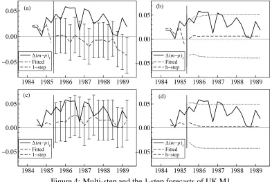
The problem with EqCMs is that they force variables back to relationships that reflect the previous equilibria—so, when equilibrium means have altered to new val-ues, EqCMs will ‘correct’ to inappropriate values. Because the new, changed, levels are disequilibria in such models, forecasts will continually be driven off course. UK M1 provides one potential example of equilibrium-mean shifts following the intro-duction in 1984 of interest-bearing retail sight deposits: these sharply lowered the opportunity costs of holding M1, shifting the long-run equilibrium mean, which, when inappropriately modeled, induced substantial forecast errors: see figs. 4a & b.

1984 1985 1986 1987 1988 1989 −0.05

0.00

0.05 (a) (b)

∆(m−p)_t

Fitted 1−step

1984 1985 1986 1987 1988 1989 −0.05

0.00 0.05

∆(m−p)_t

Fitted h−step

1984 1985 1986 1987 1988 1989 −0.05

0.00 0.05

(c)

∆(m−p)_t Fitted 1−step

1984 1985 1986 1987 1988 1989 −0.05

0.00 0.05

(d)

∆(m−p)_t Fitted h−step

Figure 4: Multi-step and the 1-step forecasts of UK M1

The forecast errors depicted here are over 1985(3)–1989(2) from an estimation sample of 1964(3)–1985(2) using a four-variable VEqCM for the logarithm of real

12 http://www.bepress.com/cas/vol3/iss2/art1

money (∆(m ₋p) in the graph denotes its first difference), the logarithm of real income (i), the rate of inflation (∆p), and the nominal interest rate (R): see Hendry (2006) for a general discussion. The bars are the 95% interval forecasts about the 1-step ahead forecasts, and the outer pair of dashed lines are the multi-period 95% interval forecasts respectively, both shown just for UK M1 although all 4 variables were forecast. The model omits the own rate of interest on M1, which only became non-zero following the legislative change in 1984. Despite in-sample congruency, well-determined estimates, and theoretically-supported cointegration in an equation for UK M1 that had remained constant for almost a decade, the 1-step forecasts are for systematic falls in real M1 during the most rapid rise that has occurred histori-cally. Almost all the forecast-horizon data lie outside the ex ante 1-step 95% interval forecasts. Such an outcome is far from ‘error correction’, prompting the renaming of cointegration combinations to equilibrium correction. Also, note that as predicted by our theory following a location shift, the multi-step forecasts are more accurate at most horizons than the 1-step, as they converge to the unconditional growth rate of real money, which remains the same as the growth rate of real income, and is not altered by the location shift.

By way of comparison, figs. 4c & d show the 1-step and multi-step forecasts respectively from precisely the same estimated model, but in first differences. This model ‘suffers from residual autocorrelation’, so its interval forecasts calculated by the usual formulae are incorrect, probably overstating the actual uncertainty. Never-theless, the absence of bias in the forecasts compared to those from the VEqCM is striking.

Consequently, VEqCMs will be reliable in forecasting only if they contain all the variables needed to track changed states of nature—here the VEqCM fails because it omits the change in the own interest rate. However, the graphs of the differenced-model forecasts of UK M1 suggest this formulation may be more robust to equilib-rium mean shifts, which is in fact a general result, as we discuss in the next section.

4.2

Location shifts and differencing

origins within a given period of time, the more likely that some of those origins will be after location shifts, allowing differenced models to outperform by their greater robustness to such shifts. This result explains the successful outcome in fig. 4b.

Care is required when calculating measures of forecast uncertainty from non-congruent models such as double-differenced forecasting devices. For example, the usual formulae for forecast-error variances can be wildly incorrect when there is substantial residual autocorrelation that is ignored (see Ericsson, 2001, for an ex-position). This stricture applies to conventionally-calculated error measures from differenced devices.

4.3

Location shifts and intercept corrections

Published macroeconomic forecasts are rarely purely model-based, and adjustments are often made to arrive at a final forecast. Such adjustments can be rationalized in a variety of ways, one of which is their role in offsetting location shifts. The last in-sample residual can be added to a model to set it ‘back on track’ (i.e., fit the last observation perfectly), and this becomes an intercept correction if it is also added to the forecast. Surprisingly, doing so changes the intercept-corrected forecasting model to a differenced form, thereby adapting immediately to any location shifts. Analysis reveals that indeed, intercept corrections have similar effects to differenc-ing in the face of location shifts, hence their empirical success.

Intercept corrections can be shown to behave similarly in the face of shifts in both equilibrium means and underlying growth rates. Forecast-error bias reductions are generally bought at the cost of less precise forecasts, so their efficacy depends on the size of location shifts relative to the horizon to be forecast. Figure 5 illustrates for UK M1. The form of intercept correction here is the same at all forecast origins, based on an average of the two errors prior to the beginning of the forecast period. The correction is only applied to the money equation, where it shifts upward the forecasts of∆(m−p), so partially corrects the under-prediction manifest in fig. 4a.

4.4

Forecast combination

The combination of forecasts is widespread in economics, at least in part because this approach has proved relatively successful in practice. There are a number of explanations as to why forecast combination works. Perhaps the most common is the ‘portfolio diversification’ argument, applicable when each individual fore-casts makes use of only a subset of all the relevant information. Newbold and Har-vey (2002) and Timmermann (2006) provide recent surHar-veys. Hendry and Clements (2004) also show that pooling forecasts can be beneficial when there are structural breaks. Clements and Hendry (2008) provide a detailed empirical illustration.

14 http://www.bepress.com/cas/vol3/iss2/art1

1984 1985 1986 1987 1988 1989 −0.04

−0.02 0.00 0.02 0.04 0.06

∆(m−p)_t Fitted 1−step

1984 1985 1986 1987 1988 1989 −0.04

−0.02 0.00 0.02 0.04 0.06

∆(m−p)_t Fitted h−step

Figure 5: Intercept-corrected forecasts of UKM1

5

Some implications

Unless the sole objective of a modeling exercise is short-term forecasting, forecast performance is not a good guide to model choice in a world of location shifts. There are no grounds for selecting the ‘best forecasting model’ for other any purposes, such as economic policy analysis, or testing economic theories. Conversely, a model may fail badly in forecasting, but its policy implications may remain correct (see Clements and Hendry, 2005).

Further, if forecast failure is primarily due to forecast-period location shifts, then there are no possible within-sample tests of later failure. The UK M1 example illus-trates this point. Whether the model breaks down after the introduction of interest-bearing checking accounts depends on how the model is updated over the forecast period–specifically, whether the interest rate variable is modified for the legisla-tive change. Forecast failure does not, though it might, entail an invalid theoretical model; it does reveal forecast data that are different from the in-sample observations, and hence an incomplete empirical model for the whole period.

they did so, then an econometric specification would also need to embody model-free forecasting rules that helped avoid systematically biased forecasts.

Finally, we have strived to explain an important facet of economic forecast-ing, namely forecast failure–which seems inevitable at the time of location shifts– although we have offered understanding, rather than solutions. An earlier and grander example is that of William Harvey’s discovery of the circulation of the blood, which led to a leap in understanding, but had no implications for heart surgery, or even blood transfusions, for several hundred years. We hope improvements to forecasting practice follow rather quicker.

References

Barrell, R. (2001). Forecasting the world economy. In Hendry, and Ericsson (2001), pp. 149–169.

Bollerslev, T. (1986). Generalised autoregressive conditional heteroskedasticity.

Journal of Econometrics, 51, 307–327.

Castle, J. L., Fawcett, N. W. P., and Hendry, D. F. (2007). Forecasting, structural breaks and non-linearities. Mimeo, Economics Department, Oxford Univer-sity.

Chatfield, C. (1993). Calculating interval forecasts. Journal of Business and

Eco-nomic Statistics, 11, 121–135.

Clements, M. P., and Harvey, D. I. (2008). Forecasting combination and encompass-ing. In Mills, T. C., and Patterson, K. (eds.), Palgrave Handbook of

Economet-rics, Volume 2: Applied Econometrics: Palgrave MacMillan. Forthcoming.

—– and Hendry, D. F. (1998). Forecasting Economic Time Series. Cambridge: Cambridge University Press.

—– and —– (1999). Forecasting Non-stationary Economic Time Series. Cambridge, Mass.: MIT Press.

—– and —– (2005). Evaluating a model by forecast performance. Oxford Bulletin

of Economics and Statistics, 67, 931–956.

—– and —– (2006). Forecasting with breaks. In Elliott, G., Granger, C., and Tim-mermann, A. (eds.), Handbook of Economic Forecasting, Volume 1.

Hand-book of Economics 24, pp. 605–657: Elsevier, Horth-Holland.

—– and —– (2008). Forecasting annual UK inflation using an econometric model over 1875–1991. In Rapach, D., and Wohar, M. (eds.), Forecasting in the

Presence of Structural Breaks and Model Uncertainty. Frontiers of Economics and Globalization. Volume 3: Elsevier, Horth-Holland. Forthcoming.

16 http://www.bepress.com/cas/vol3/iss2/art1

Davidson, J. E. H., Hendry, D. F., Srba, F., and Yeo, J. S. (1978). Econometric mod-elling of the aggregate time-series relationship between consumers’ expendi-ture and income in the United Kingdom. Economic Journal, 88, 661–692. Eitrheim, Ø., Husebø, T. A., and Nymoen, R. (1999). Equilibrium-correction versus

differencing in macroeconometric forecasting. Economic Modelling, 16, 515– 544.

Engle, R. F. (1982). Autoregressive conditional heteroscedasticity, with estimates of the variance of United Kingdom inflation. Econometrica, 50, 987–1007. Ericsson, N. R. (2001). Forecast uncertainty in economic modeling. in Hendry, and

Ericsson (2001), pp. 68–92.

Hendry, D. F. (1995). Econometrics and business cycle empirics. Economic Journal,

105, 1622–1636.

—– (2004). The Nobel Memorial Prize for Clive W.J. Granger. Scandinavian

Jour-nal of Economics, 106, 187–213.

—– (2006). Robustifying forecasts from equilibrium-correction models. Journal of

Econometrics, 135, 399–426.

—– and Clements, M. P. (2004). Pooling of forecasts. The Econometrics Journal,

7, 1–31.

—– and Ericsson, N. R. (eds.)(2001). Understanding Economic Forecasts. Cam-bridge, Mass.: MIT Press.

—– and Juselius, K. (2000). Explaining cointegration analysis: Part I. Energy

Journal, 21, 1–42.

—– and —– (2001). Explaining cointegration analysis: Part II. Energy Journal, 22, 75–120.

—– and Nielsen, B. (2007). Econometric Modeling: A Likelihood Approach. Prince-ton: Princeton University Press.

Kuhn, T. (1962). The Structure of Scientific Revolutions. Chicago: University of Chicago Press.

Makridakis, S., and Hibon, M. (2000). The M3-competition: Results, conclusions and implications. International Journal of Forecasting, 16, 451–476.

Newbold, P., and Harvey, D. I. (2002). Forecasting combination and encompass-ing. In Clements, M. P., and Hendry, D. F. (eds.), A Companion to Economic

Pesaran, M. H., and Skouras, S. (2002). Decision-based methods for forecast evalu-ation. In Clements, M. P., and Hendry, D. F. (eds.), A Companion to Economic

Forecasting, pp. 241–267: Oxford: Blackwells.

Singer, M. (1997). Thoughts of a nonmillenarian. Bulletin of the American Academy

of Arts and Sciences, 51(2), 36–51.

Timmermann, A. (2006). Forecast combinations. In Elliott, G., Granger, C., and Timmermann, A. (eds.), Handbook of Economic Forecasting, Volume 1.

Handbook of Economics 24, pp. 135–196: Elsevier, Horth-Holland.

Todd, R. M. (1990). Improving economic forecasts with Bayesian vector autoregres-sion. In Granger, C. W. J. (ed.), Modelling Economic Series, Ch. 10. Oxford: Clarendon Press.

West, K. D. (2006). Forecasting evaluation. In Elliott, G., Granger, C., and Timmer-mann, A. (eds.), Handbook of Economic Forecasting, Volume 1. Handbook of

Economics 24, pp. 99–134: Elsevier, Horth-Holland.

18 http://www.bepress.com/cas/vol3/iss2/art1