A Thesis Submitted for the Degree of PhD at the University of Warwick
http://go.warwick.ac.uk/wrap/50020
This thesis is made available online and is protected by original copyright. Please scroll down to view the document itself.
Reflected Brownian Motion
by
Janosch Ortmann
Thesis
Submitted to The University of Warwick
for the degree of
Doctor of Philosophy
Abstract v
Acknowledgments vi
Declaration viii
List of Notation ix
1 Introduction 1
2 Background Material 5
2.1 Catalan Structures and Combinatorics . . . 5
2.1.1 Dyck Paths and Non-Crossing Partitions . . . 5
2.1.2 Lattices, Parking Functions and Permutations . . . 8
2.1.3 Block Structure for Non-Crossing Partitions . . . 9
2.2 Free Probability Theory . . . 12
2.2.1 Non-Commutative Probability Spaces . . . 12
2.2.2 Freeness and Combinatorics . . . 14
2.2.3 Analytic Aspects and Transforms . . . 17
2.2.4 Semicircular Processes . . . 19
2.2.5 Law of Large Numbers and Central Limit Theorem . . . 20
2.2.6 The Full Fock Space, Creation and Annihilation . . . 22
2.2.7 Free Probability and Random Matrix Theory . . . 23
2.2.8 Free Brownian Motion and Bridge . . . 25
2.3 Large Deviations Theory . . . 27
2.3.1 Basic Notions . . . 27
2.3.2 Contraction principles . . . 30
2.3.3 Cram´er’s Theorem and Sanov’s Theorem . . . 32
2.3.4 Projective Limits . . . 36
2.4 Reflected BM and Queuing Theory . . . 37
2.4.1 RBM in a Polyhedral Domain . . . 37
2.4.2 RBM in an Orthant . . . 39
2.4.3 Queuing Networks . . . 40
3 Large Deviations for Non-Crossing Partitions 43
3.1 Introduction . . . 43
3.2 Process Level Large Deviations . . . 44
3.2.1 Joint Sanov and Cram´er . . . 45
3.2.2 The Sample-Path Result . . . 51
3.3 Construction of the Uniform Measure on NC(n) . . . 54
3.4 Large Deviations for Non-Crossing Partitions . . . 56
3.4.1 The Upper Bound . . . 57
3.4.2 The Lower Bound . . . 60
3.5 A Formula for the Maximum of the Support . . . 64
3.5.1 All Free Cumulants Positive . . . 66
3.5.2 Non-Negative Free Cumulants . . . 68
3.6 Examples . . . 69
3.6.1 Freely Infinitely Divisible Distributions . . . 71
3.6.2 Series of Free Random variables . . . 72
4 Functionals of the Free Brownian Bridge 75 4.1 Series Representations for the Bridge . . . 75
4.2 Square Norm of the Free Brownian Bridge . . . 77
4.2.1 The R-transform . . . 78
4.2.2 Free Infinite Divisibility . . . 80
4.2.3 The Maximum of the Support . . . 83
4.3 The Signature of the Free Brownian Bridge . . . 84
4.3.1 Signature and Rough Paths . . . 84
4.3.2 Using the L´evy Representation . . . 86
4.3.3 The Distribution of the Tensor Product and Meanders . . . . 86
4.3.4 The Distribution of the Signature . . . 90
4.4 L´evy Area of the Free Brownian Bridge . . . 93
5 Analogues of Reflected Brownian Motion 98 5.1 Generalised RBM . . . 98
5.2 Main Results . . . 100
5.2.1 GRBM in a General Domain . . . 100
5.2.2 General Covariance . . . 102
5.3 Examples . . . 103
5.3.1 One-Dimensional ERBM and Dufresne’s Identity . . . 103
5.3.2 RBM in a Weyl Chamber . . . 104
5.3.3 Examples Motivated by Queueing Theory . . . 105
5.4 Proofs of the Main Results . . . 108
5.4.1 General Polyhedral Domain . . . 109
5.4.2 Orthant with General Covariance . . . 111
A Computations for the Square Norm 113 A.1 Unique Solution in Polar Co-Ordinates . . . 113
A.1.1 First Case: t∈(π,32π). . . 115
A.1.3 Third, and Last Case: t∈5π
3 ,2π
. . . 121 A.2 Solving the Variational Problem . . . 123
In this thesis we present results in large deviations theory, free probability and the theory of reflected Brownian motion.
We study the large deviations behaviour of the block structure of a non-crossing partition chosen uniformly at random. This allows us to apply the free moment-cumulant formula of Speicherto express the spectral radius of a non-commutative random variable in terms of its free cumulants.
Next the distributions of three quadratic functionals of the free Brownian bridge are studied: the square norm, the signature and the L´evy area of the free Brown-ian bridge. We introduce two representation of the free BrownBrown-ian bridge as series involving free semicircular variables, analogous to classical results due to L´evy and Kac. The latter representation extends to all semicircular processes. For each of the three quadratic functionals we give the R-transform, from which we extract in-formation about the distribution, including free infinite divisibility and smoothness of the density. We also apply our result about the spectral radius to compute the maximum of the support for L´evy area and square norm. In both cases we obtain implicit equations.
The final chapter of the thesis is devoted to the study of a generalisation of reflected Brownian motion (RBM) in a polyhedral domain. This is motivated by recent developments in the theory of directed polymer and percolation models, in which existence of an invariant measure in product form plays a role. Informally, RBM is defined by running a standard Brownian motion in the polyhedral domain and giving it a singular drift whenever it hits one of the boundaries, kicking the process back into the interior. Our process is obtained by replacing this singular drift by a continuous one, involving a continuous potential. RBM has an invariant measure in product form if and only if a certain skew-symmetry condition holds. We show that this result extends to our generalisation. Applications include examples motivated by queueing theory, Brownian motion with rank-dependent drift and a process with close connections to the δ-Bose gas.
First and foremost I would like to thank my supervisor, Neil O’Connell for all his inspiration, support and guidance over the last three and a quarter years. He has been incredibly generous with his time and his inspiration, and I could not have wished for a better mentor.
I would also like to thank Philippe Biane and Jon Warren, for agreeing to be my examiners. Their detailed comments and corrections have allowed me to remove many errors and inaccuracies and improve this thesis considerably.
Jon Warren and Nikos Zygouras have listened to a talk I gave based on earlier versions of part of this thesis, and I would like to thank them for their input and suggestions.
Thanks are also due to Octavio Arizmendi, Philippe Biane, Ion Nechita, Roland Speicher, Jon Warren and Nikos Zygouras for invaluable discussions and suggestions concerning various parts of this thesis.
I am very grateful to Lionel Mason and Giovanna Scataglini-Belghitar for their guidance when I was an undergraduate, to Bal´azs Szendr¨oi and Geoffrey Nicholls for many interesting tutorials, and to Alison Etheridge for getting me into probability theory.
Closer to home I would like to thank my mother, der diese Arbeit gewidmet ist, and Kolja Ortmann, for always being there. Finally, Flavie Sch¨afer, for considerably more than I could say here.
The author declares that the material contained in this thesis is entirely his own work, with the exception of the material in Chapter 5, which arose from joint work with NeilO’Connell. As is standard practice, the subject matter developed builds on existing theory, and clear citations and references are provided where necessary.
No part of this thesis has been submitted, for the purposes of a degree or other-wise, to any other university or educational institution.
The material in Chapter 3 has been accepted for publication to the Electronic Journal of Probability, under the title Large deviations for non-crossing partitions
[91].
Chapter 4 is based on the paper Functionals of the free Brownian bridge [90] by the author, which has been submitted to the S´eminaires de probabilit´es.
The results in Chapter 5 will appear in the paper Product-form invariant mea-sures for Brownian Motion with drift satisfying a skew-symmetry type condition [87].
Abbreviations
Z the set of integers
N the set of natural numbers
N0 the set of non-negative integers,N0 =N∪ {0}.
D(I, E) the space of c`adl`ag functions from an intervalI ⊂R to a topological space E.
C(E) the space of continuous real-valued functions on a topological space E
Cb(E) the subspace ofC(E) consisting of all bounded functions
S1 the unit circle inR2
M+(E) the set of positive finite measures on a topological space E with
its Borel σ-algebra
Ms(E) the subset of µ∈M+(E) such that µ(E) = s, for some s∈(0,∞)
δx the Dirac measure concentrated onx
mk(µ) the kth moment of a measure µon R.
|x| the Euclidean norm of a vectorx∈Rd.
i.i.d. independent and identically distributed
τ(V0, V) the coarsest topology on the algebraic dual of a vector space V0 with respect to which the maps f 7−→f(x) are continous for all x∈V.
Unless otherwise stated we equip sets of measures with the weak topology.
Introduction
The theory of free probability was introduced byVoiculescu[123, 124, 125], origi-nally as a tool in operator algebras, in order to study type II von Neumann algebras. Its two central ingredients are the concept of a non-commutative probability space on the one hand and a new type of independence, based on free rather than tensor products, on the other.
Probabilists’ interest stems from the fact that random matrices can naturally be considered as non-commutative random variables and that many ensembles studied in random matrix theory are asymptotically free, that is, they become free as the size of the matrix tends to infinity. This allows one to compute joint asymptotic spectral distributions.
More recently free probability theory has also proved a useful tool in wireless communications [64, 77, 79, 118, 119], quantum information theory [5, 7] and the study of randomly disordered systems, in connection with the Anderson model [80, 110].
In all of these areas the R-transform is a powerful tool for computations. Given an R-transform we can, at least in theory, obtain the corresponding probability measure. However in order to do so one needs to find the functional inverse of the R-transform for which a closed-form expression may not exist. This raises the
question what information can be inferred from the R-transform without inverting it. In Chapter 3 we present a formula for the right edge of the support of a probability measure in terms of its free cumulants.
As a key ingredient we establish a large deviations principle for the block struc-ture of uniformly random non-crossing partitions. A law of large numbers, stating that the proportion of blocks of size ktends to 2−kas the sizen of the set to be par-titioned goes to infinity, follows. This result in random combinatorics, in the spirit of [27, 35, 121], can be extended, via well-chosen bijections, to other combinatorial structures, including the descents of Dyck paths, the lengths of chains in ordered trees and the blocks of non-nesting partitions.
The large deviations result allows us to apply Varadhan’s lemma to Speicher’s free moment-cumulant formula in order to express the right edge of the support of a probability measureµas a variational formula involving its free cumulants, provided these are non-negative.
The semicircle law, which arises as the asymptotic spectral distribution of Wigner matrices [129] is in many ways the free analogue of the Gaussian distribution. We have the concept of a semicircular process, of which the free Brownian motion is a prominent example. It can be considered as the limit of Brownian motion on the space of N ×N Hermitian matrices as the size N tends to infinity. From the free Brownian motion we obtain the free Brownian bridge in the same way as in classical probability theory. In Chapter 4 we introduce two representations of the free Brownian bridge as series of freely independent semicircular random variables, one of which extends easily to all semicircular processes.
densities with respect to Lebesgue measure and give implicit equations for the den-sity. Using the spectral radius result from Chapter 3 we also compute the right edge of the support. For the signature a connection with certain combinatorial objects called irreducible meanders appears somewhat unexpectedly.
There has been much recent development on the study of positive-temperature per-colation and polymer models [33, 84, 88, 103, 104]. These turn out to be closely related to random matrix theory on the one hand and the study of the KPZ equa-tion [58], which was proposed to describe a class of surface growth models, on the other. An important role is played by an exactly solvable discrete directed percola-tion model which was introduced in [89] and further studied in [26, 76, 84, 104, 111]. In [84] the partition function of the polymer model is related to a diffusion process whose generator is given in terms of the Hamiltonian of the quantum Toda lattice. The proof uses a multi-dimensional generalisation of results by Matsumoto–Yor [68, 69, 71], concerning exponential functionals of Brownian motion. For connec-tions between these models, Whittaker funcconnec-tions and representation theory we refer to the recent survey [86].
The polymer model introduced in [89] can also be viewed as a network of gen-eralised Brownian queues in tandem. A crucial role is played by an analogue of the output or Burke theorem, which states that the output of the M/M/1 queue up to a fixed time t is independent of the queue length at time t. This leads to a product-form invariant distribution for the series of queues.
Queueing networks [34, 50, 51, 96] provide examples of reflected Brownian mo-tion (RBM) in a polyhedral domain, introduced and studied by Harrison and
Motivated by this we introduce a multidimensional diffusion we call generalised RBM (GRBM). Rather than giving the Brownian motion a singular drift whenever it hits one of the boundaries, we now impose a continuous drift. Its magnitude depends, via a potential U, on the position of the process relative to the polyhedral domain. A special case, the exponentially RBM, corresponds to the choice U(x) = −e−x, which corresponds to the generalised Brownian queue.
We show that for the GRBM existence of an invariant measure in product form is still equivalent to the skew-symmetry condition of Harrison–Williams, inde-pendent of the function U.
By introducing a parameter β (which can be viewed asinverse temperature) and lettingβ −→ ∞, we recover the diffusion studied byHarrison–Williams. In this sense our process really is a generalisation of reflected Brownian motion.
Apart from examples motivated by queueing networks we also study the analogue of Brownian motion with rank-dependent drift [92] and draw connections to the δ -Bose gas recently studied and related to reflected Brownian motion byProlhac–
Background Material
This chapter is devoted to those aspects of combinatorics, large deviations theory, free probability theory and reflected Brownian motion that we require later on.
2.1
Catalan Structures and Combinatorics
We present here some background on combinatorics, in particular Catalan struc-tures. Our focus will lie on non-crossing partitions and Dyck paths.
2.1.1
Dyck Paths and Non-Crossing Partitions
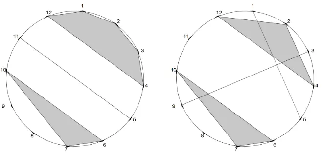
Definition 2.1.1. A partition π of the set n = {1, . . . , n} is said to be crossing if there exist distinct blocks V1, V2 of π and xj, yj ∈Vj such that x1 < x2 < y1 < y2.
Otherwise π is said to be non-crossing. Equivalently, label the vertices of a regular
n-gon 1, . . . , n then π is non-crossing if and only if the convex hulls corresponding to the blocks are pairwise disjoint. We denote the set of all non-crossing partitions of n by NC(n).
Non-crossing partitions were first introduced by G. Kreweras [60] and has first attracted attention from combinatorialists. Later they have also been studied in connection with low-dimensional topology and geometric group theory, symmetric
groups [72], algebraic combinatorics and mathematical biology [93, 105]. We will explore in some detail further connections with parking functions and free probability theory.
Figure 2.1: The partition {{8},{9},{10,7,6},{11,5},{12,4,3,2,1}}
is non-crossing,{{5,1},{8},{9,3},{10,7,6},{12,4,2}}is crossing.
A Dyck path of semilength n is a lattice path in Z2 that never falls below the
horizontal axis, starting at (0,0) and ending at (2n,0), consisting of steps (1,1) (upsteps) and (−1,1) (downsteps). Every such path consists of exactly n up- and downsteps each. The set of Dyck paths of semilengthn is denoted byP(n). A max-imal sequence of upsteps is called anascent, while a maximal sequence of downsteps is referred to as a descent.
The cardinalities of P(n) and NC(n) are both given by the nth Catalan number
Cn=
1
n+ 1
2n n
.
(n+ 2)-gons, binary trees withn vertices and pairs of standard Young tableaux of the same shape, consisting ofn squares and at most 2 rows. A long list of examples was compiled byStanley[114] (Exercise 6.1.9), where many results and references on Catalan structures can also be found.
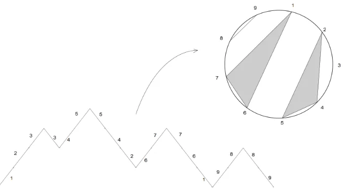
There is a well-known bijection Φ : P(n)−→NC(n) which maps the descents of
p ∈ Pn to the blocks of Φ(p) [30, 131]. Given p ∈ Pn label the upsteps from left
to right by 1, . . . , n. Label each downstep by the same index as its corresponding upstep, that is the first upstep to the left on the same horizontal level. Then the descents induce an equivalence relation onn: two labels are equivalent if and only if the corresponding downsteps are part of the same descent. The associated partition is then easily seen to be non-crossing.
Conversely, given π={V1, . . . , Vr} ∈NC(n) write the elements of each blockVj
[image:17.595.146.495.476.673.2]in descending order, then sort the blocks in ascending order by their largest elements. This gives the descent structure of Φ−1(π), which can be complemented by ascents in a unique way to form a Dyck path.
Figure 2.2: An example for the bijection Φ.
other bijections which map the blocks of a non-crossing partition to an interesting substructure. We mention here the lengths of chains in ordered trees [94] and the blocks of non-nesting partitions [97].
As a small generalisation let us mention the k-divisible non-crossing partitions for somek ∈N. A non-crossing partition of the setm is said to be k-divisible if the size of each block is divisible by k. Of course such a partition can only exist if m
is a multiple of k and we denote by NC(k)(n) the set of all k-divisible non-crossing partitions of kn. The image of NC(k)(n) under the bijection Φ described above can be identified [6] with the set of k-Dyck paths, i.e. the paths with upsteps (1,1) and downsteps (1,−k). The cardinality of NC(k)(n) is given [44] by the Fuss-Catalan numbers
NC(k)(n) = 1
n
(k+ 1)n n−1
.
See Armstrong [3] for a survey of a more general object on Coxeter groups.
2.1.2
Lattices, Parking Functions and Permutations
The set of non-crossing partitions can be given a partial order(called the reverse refinement order) defined by setting π σ if and only if every block of π is com-pletely contained in one of the blocks of σ. The maximal element of NC(n) with respect to this order is the partition 1n with a single equivalence class. The partition
consisting of n singleton blocks, denoted 0n, is the minimal element. By
Proposi-tion 9.17 in Nica–Speicher[83], the partial order induces alattice structure on NC(n), that is for any π, σ ∈NC(n) there exists
(i) a join π∨σ, that is an element τ ∈ NC(n) such that τ σ and τ π that has τ τ0 for any other τ0 with that property
The lattice of non-crossing partitions can also be embedded into the Cayley graph of the symmetric group Sn. This map, due to Biane [17] allows us to relate our
large deviations result to the cycle structure of the permutations lying on a geodesic from the identity element in Sn to the maximal cycle (1. . . n).
A geodesic between two points a, b on any non-oriented graph G = (V, E) is a path froma tob inG of minimal length. For verticesv1, v2 we denote by [v1, v2] the
set of vertices of G that lie on some geodesic from v1 tov2. This is an ordered set,
indeed another lattice, withw1 ≤w2 if and only if w1 lies on some geodesic fromv1
to w2.
IfGis the Cayley graph ofSnwith the collection of all transpositions as generator
set then [17] gives an order-preserving bijection Ψ from [e,(1. . . n)] to NC(n). The map Ψ is given by associating to a permutation the partition given by its cycle structure. In particular Ψ maps bijectively the cycle structure of [e,(1. . . n)] to the block structure of NC(n), so we get a large deviations principle, of speednand with rate function J given above, for the cycle structure of uniformly random elements of [e,(1. . . n)].
In [18] P. Biane uses this bijection to re-derive a bijection between maximal chains in the lattice NC(n+ 1) and parking functions onn, originally established by
Stanley [113]. A parking function is a sequence of natural numbers (a1, . . . , an)
such that its increasing rearrangement (a(1), . . . a(n)) has a(j) ≤j for all j.
2.1.3
Block Structure for Non-Crossing Partitions
We survey here previously known enumerative and asymptotic results about the block structure of non-crossing partitions. For a given π ∈ NC(n) we denote by
Bk(π) the number of blocks of size k in π, and byB(π) the total number of blocks
of π.
each j ∈n is given [60] by
n! Qn
j=1rj!
n+ 1−Pn
j=1rj
!
.
The number of non-crossing partitions of n with k blocks is given [40] by the
Narayana numbers
N(n, k) = 1
n
n
k
n
k−1
.
Therefore the expected number of descents in w is n+12 . One could also deduce this latter fact using the Kreweras complement K: NC(n) −→ NC(n), which is defined as follows: consider additional numbers 1, . . . , n and interlace them with 1, . . . , n so that j lies between j and j + 1. Then the Kreweras complement K(π) of π ∈NC(N) is the biggest element (with respect to the inverse refinement order) of those σ ∈ NC(1, . . . , n) with the property that the partition π ∪ σ of the set {1,1, . . . , n, n), formed by taking all the blocks of π and all those of σ together, is
non-crossing. Then [83] K is a lattice anti-isomorphism (i.e. a bijection such that
σ π implies K(σ)K(π) such that for any π ∈NC(n),
B(π) +B K π =n+ 1.
From this it follows directly that the expected number of blocks is n+12 .
Let furtherT(n, k) denote the number ofπ ∈NC(n) withk singleton blocks and denote its generating function by G(t, z), then [131, p.3153]
G(t, z) = ∞ X
n=1
∞ X
k=0
T(n, k)tkzn= 1 + (1−t)z− p
1−2(1 +t)z+ (2t+t2−3)z2
Denote the total number of singletons in all π ∈NC(n) by αn, then
∞ X
n=1
αnzn =
∞ X
n=1
n
X
k=0
kT(n, k)zn = ∂
∂tG(t, z)
t=1
= √ z 1−4z =
∞ X
n=0
2n n
z
n+1
.
So the expected number of singletons in a non-crossing partition chosen uniformly at random is given by
1
Cn
2n−2
n−1
=
n2+n
4n−4 '
n
4.
2.2
Free Probability Theory
We dicuss here some concepts and results from free probability theory. More on the subject can be found, for example, in the books [55, 127, 128] and the survey aimed at probabilists by Biane [19]. For the concepts in classical probability that we mention we refer to the books [98, 100, 101].
2.2.1
Non-Commutative Probability Spaces
Before defining the basic object of study in free probability we need to recall some notions from functional analysis. More details can be found in the book byMurphy [78].
Definition 2.2.1. A complex algebraAwith unit1A and an involution∗:A −→ A such that 1∗A =1A is said to be a ∗-algebra. A ∗-algebra equipped with a norm k·k is called a C∗-algebra if A is complete with respect to k·k, k1Ak = 1 and for all
a, b∈ A we have
ka∗k=kak, ka∗ak=kak2, kabk ≤ kak
Elements a ∈ A are said to be normal if a∗a = aa∗, self-adjoint if a∗ = a and
positive if there exists self-adjoint b∈ A such thata=b2.
Definition 2.2.2. A non-commutative probability space is a ∗-algebra A together with a state φ, that is a linear functional φ: A −→ C such that φ(1A) = 1 and
φ(a)≥0 whenever a is positive.
Whenever topological concepts like convergence are involved we will additionally assume that (A, φ) is a C ∗-probability space, that is A is a C∗-algebra andφ
We think of elements a∈ A as non-commutative random variables and consider
φ(a) to be the expectation ofa ∈ A. This is motivated by the fact that for a classical probability space (Ω,F,P) the spaceAof bounded complex-valued random variables equipped with the state A 3 X 7−→ E(X) ∈ C is a non-commutative probability space in the sense of our definition.
If a ∈ A is self-adjoint there exists a compactly supported measure µa on R, called the distribution of a, such that
φ(an) = Z
tnµa(dt) ∀n∈N.
The existence of a distribution is analogous to classical probability theory. We note, however, that in our setting the distribution is always compactly supported. In this sense we are therefore only considering bounded random variables. There is a theory of unbounded non-commutative random variables, using affiliated elements of operator algebras, but we do not require this here and instead refer to the papers by Maassen [67] and Bercovici–Voiculescu [13].
Example 2.2.3. Let (Ω,F,P) be a classical probability space, fix N ∈ N and let AN be the algebra of N ×N random matrices with all moments, that is N ×N
matrices whose entries are elements of
L∞−(Ω,F,P) = \
p≥1
Lp(Ω,F,P).
Equipped with the state φN given by φN(a) = EtrN(a) (where trN denotes the
µa of a is then characterised by its action on continuous test functionsf ∈ C(R):
Z
fdµa=
1
N
N
X
j=1
E[f(λj)].
Note that ifa∈ AN is self-adjoint the eigenvaluesλ1, . . . , λN of aare real and hence
the support of µa is a subset of the real line.
Example 2.2.4. Let H be a complex separable Hilbert space and fix h ∈ H with khk = 1. Let A = B(H), the C∗-algebra of bounded operators on H. Equipped
with the faithful normal trace φ given by
φ(a) =ha(h), hi
the pair (A, φ) is a non-commutative probability space. In fact, by the GNS
con-struction [78], every non-commutative probability space can be realised in this way. See also Section 2.2.6.
2.2.2
Freeness and Combinatorics
Having introduced non-commutative probability spaces we now turn to the second ingredient in free probability: free independence. We discuss this following the combinatorial approach by Speicher [107, 108, 109], relying on the presentation by Biane [19]. See also Nica–Speicher [81, 83]. An analytic approach to free probability will be presented in Section 2.2.3 below.
Definition 2.2.5. C∗-subalgebrasB1, . . . ,BN ofAare said to be freely independent,
orfree, if for every set of indices{rj}mj=1 ⊆ {1, . . . , N} and collection{aj ∈ Brj: 1≤ j ≤m}such that rj 6=rj+1 and φ(aj) = 0 ∀j we already have
Random variables a1, . . . , aN are said to be free if the unital C∗-algebras generated
by the aj are free.
Suppose a1, a2 ∈ A are free. Then we can calculate directly the joint moments of
the aj. For example:
φ(a1a2) =φ(a1)φ(a2) (2.2.6)
φ(a1a2a1a2) =φ(a1)2φ(a22) +φ(a 2
1)φ(a2)2 −(φ(a1)φ(a2)) 2
. (2.2.7)
In fact, all joint moments of a1, a2 are determined by the restriction of φ to the
subalgebras A1 = A(1, a1), A2 = A(1, a2). This compares well with the fact that
we can calculate the joint distribution of an independent family of independent classical random variables given their marginal distributions. However, trying to find explicit formulae for higher moments by hand quickly leads to complicated formulae. This was elegantly solved by combinatorial means by R. Speicher.
Definition 2.2.8. Thefree cumulants ofAare defined to be the mapskn: An−→C
(n∈N) defined indirectly by the following system of equations:
φ(a1, . . . , an) =
X
π∈NC(n)
kπ[a1, . . . , an] (2.2.9)
where kπ denotes the product of cumulants according to the block structure of π.
That is, if V1, . . . , Vr are the components of π ∈NC(n) then
kπ[a1, . . . , an] =kV1[a1, . . . , an]. . . kVn[a1, . . . , an]
where, for V = (v1, . . . , vr) we just have kV[a1, . . . , an] =k|V|[av1, . . . , avr].
Note that (2.2.9) has the form φ(a1, . . . , an) =kn[a1, . . . , an]+ lower order terms, so
inversion. This fits in a larger frameworks of multiplicative functions on lattices of partitions, which is explained in [83].
Because of the definition and the fact that φ is linear it follows that for each n
the function kn isn-multilinear in its arguments.
We will writekn(a) forkn(a, . . . , a). TheR-transform of a random variablea ∈ A
is defined, as formal power series, by
Ra(z) =
∞ X
n=0
kn+1(a)zn. (2.2.10)
Theorem 2.2.11. For a1, . . . , an∈ A the following two conditions are equivalent:
(i) a1, . . . , an are free,
(ii) mixed cumulants vanish: for all n ≥ 2 we have, whenever i(1), . . . , i(m) ∈ n
such that there exist p, q ∈n with i(p)6=i(q),
km ai(1), . . . , ai(m)
= 0.
Corollary 2.2.12. If a, b∈ A are free then for all n ∈N we have
kn(a+b) = kn(a) +kn(b).
So, if a1 and a2 are free, then the distribution of a1+a2 is uniquely determined by
those of a1 and a2.
For each pair of probability measures µ1, µ2 with compact support there exist a
non-commutative probability space (A, φ) and free a1, a2 ∈ A such that the
distri-bution ofaj isµj. So we get a binary operation on the space of compactly supported
probability measures, called free convolution and denoted .
vari-able.
Proposition 2.2.13. For a ∈ A we have the following formula:
φ(an) = X
π∈NC(n)
kπ. (2.2.14)
On the level of formal power series [112] we have the following relation between the Cauchy transform Gµa of µa,
Gµa(z) =
Z
µ(dt)
z−t =
∞ X
n=0
φ(an)z−n−1
and the R-transform of a:
Corollary 2.2.15. Let a ∈ A and G, R denote its Cauchy and R-transforms re-spectively. Considering these as formal power series we have
G
R(z) + 1
z
=z.
2.2.3
Analytic Aspects and Transforms
In contrast to the combinatorial approach with generating functions described above we now describe certain analytic considerations, using holomorphic functions. Through-out this section fix an elementa of a non-commutative probability space (A, φ) and denote its distribution by µa.
Since µa is compactly supported, the Cauchy transform Gµa defines an analytic
map from C+ into C−, which extends analytically to a neighbourhood Ua of ∞.
Rather than as a formal power series we can now consider the right-hand side as a holomorphic power series, valid onUa. We will also write Ga for Gµa.
function on a neighbourhood of zero [55, Theorem 3.2.1]. Moreover the Cauchy transformGaofais locally invertible on a neighbourhood of infinity and the inverse
Ka satisfies
Ka(z) =Ra(z) +
1
z.
Remark 2.2.16. Using the continuity of φ and multilinearity of the cumulants we now obtain the following properties of the R-transform:
1. Ifanconverges toain the operator topology ofAthen there exists a
neighbour-hood U of zero where Rn, R are defined for all n ∈ N and Ran(z) −→ Ra(z)
as n→ ∞ for every z ∈U.
2. If a, b∈ A are free then Ra+b(z) =Ra(z) +Rb(z)
3. Forλ ∈Cwe have Rλa(z) =λRa(λz).
So the R-transform plays the role of the logarithm of the Fourier transform in classical probability theory: it is linear, additive on (freely) independent random variables, and determines the underlying distribution. Moreover its Taylor coeffi-cients are also related to the moments by summing over a lattice of partitions: in the classical case over all, in the free case over the non-crossing partitions.
However, in contrast to the Fourier transform, it is not straightforward to read off properties of µfrom its R-transform. The most direct way is to find the Cauchy transform (by inverting Rµ(z) + 1z) and the applying Stieltjes inversion [55, p. 94]:
Theorem 2.2.17. Let µbe a compactly supported probability measure them
µ= lim
y↓0
−1
πImGµ(x+iy)
where the limit is in the weak topology on M1(R). Moreover t0 ∈ R is an isolated
point of the support of µ if and only if Gµ can be extended meromorphically to a
neighbourhood of t0 such that this extension has a simple pole at t0. When µ has a
continuous density f with respect to Lebesgue measure then
f(x) =−1
π limy↓0Gµ(x+iy).
2.2.4
Semicircular Processes
Definition 2.2.18. A collection S = (sj)j∈I of non-commutative variables on A is
said to be a semicircular family with covariance (c(i, j))i,j∈I if the cumulants are given by
kπ[sj1, . . . sjn] =
Q
p∼πqc(jp, jq) if π is a pair partition
0 otherwise.
If S consists of a singleton s1 and r = 2
p
c(1,1) then the distribution of s1 is the
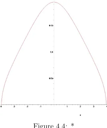
centred semicircle law of radius r, that is the measure σr onR given by
σr(dt) =
2
πr2
√
r2−t2 1
[−r,r](t) dt.
In particular σ2 is also called the standard semicircle law and non-commutative
random variables with law σr (σ2) are referred to as(standard) semicirculars.
radius r is given by
R(z) = r
2
4 z.
Recall that the centred Gaussian distribution is characterised by the fact that only the second classical cumulant is nonzero.
Moreover a collection of random variables with a joint semicircular law is deter-mined by its covariance. To be more precise we recall the following
Proposition 2.2.19(Nica–Speicher[83], Proposition 8.19). Let(si)i∈Ibe a
semi-circular family of covariance (c(i, j))i,j∈I and suppose I is partitioned by I1, . . . , Id.
Then the following are equivalent:
1. The collections {sj: j ∈I1}, . . . ,{sj: j ∈Id} are free
2. We have c(r, j) = 0 whenever r∈Ip and j ∈Iq with p6=q.
In particular {sj: j ∈I} is a free family if and only ifC = (c(r, j))r,j∈I is diagonal.
Definition 2.2.20. A process (X(t))t≥0 onAis said to be a semicircular process if
for every t1, . . . , tn ∈[0,∞), the set (X(t1), . . . , X(tn)) is a semircular family.
By the considerations above the finite-dimensional distributions of a semicircular process are determined by the covariance structure of the process, i.e. by the func-tion C: [0,∞)2 −→
C defined by
C(s, t) =φ(X(s)X(t)).
.
2.2.5
Law of Large Numbers and Central Limit Theorem
only a single variable is involved, we can no longer use measure theory (because of non-commutativity) and are forced to work with moments only. Recall that for a single non-commutative random variable convergence in distribution is equivalent to convergence in moments.
Let ChX1, . . . , XNi denote the algebra of non-commutative polynomials in the
variables X1, . . . , XN.
Definition 2.2.21. Leta1, . . . aN ∈ Afor some non-commutative probability space
A. The linear functional µa1,...,aN: ChX1, . . . , XNi −→C defined by
µa1,...,aN P x1, . . . , xN
=φ(P (a1, ldots, aN))
is called the joint distribution of a1, . . . aN.
Definition 2.2.22. Let I be a finite set. For each n ∈ N let naj(n):j ∈Io be a family of random variables in a noncommutative probability space (An, φn) with
joint distribution µn. The family of random variables is said to converge in (joint)
distribution toa1, . . . , aN for some non-commutative probability space (A, φ) if the
joint distribution of a1, . . . , aN isµ and
lim
n→∞µn(P) = µ(P) ∀P ∈Ch{Xj: j ∈I}i.
A law of large numbers for free random variables was established byBercovici–
Pata[11]. We state it here in the context of self-adjoint random variables with real, compact support and refer to [11] the statement in full generality.
Theorem 2.2.23. Let (Xn)n∈N be a sequence of free identically distributed random
variables whose common distribution µ is compactly supported in R. Then the
non-commutative law of 1
n
Pn
k=1Xk converges weakly to a point mass at m1(µ).
It can be verified directly using free cumulants. For details we refer to [128] or Chapter 8 of [83].
Theorem 2.2.24 (Free Central Limit Theorem). Let (aj)j∈N be a free family of
random variables such that
(i) φ(aj) = 0 for all j ∈N;
(ii) supj∈
N
φ(akj)
<∞ for all k ∈N;
(iii) limn→∞ n1 Pnj=1φ a2j
=r2/4.
Then the sequence (sn)n∈N of random variables defined by
sn =
1
n
n
X
j=1
aj
converges in non-commutative distribution to the centred semicircle law of radius r.
2.2.6
The Full Fock Space, Creation and Annihilation
In order to deal with convergence issues it will be useful to choose a specific non-commutative probability space. LetH0be an infinite-dimensional separable complex
Hilbert space and define the full Fock space to be
T ((H0)) =
∞ M
n=0
H⊗n
0 (2.2.25)
where by convention H⊗00 = CΩ for a distinguished unit vector Ω. Equip the C∗ -algebra B(T ((H0))) of continuous linear functionals on T ((H0)) with the tracial
state φ given by
Definition 2.2.27. For h ∈ H0 define the creation and annihilation operators to
be l(h) andl∗(h) respectively where
l(h)(h1⊗. . .⊗hn) = h⊗h1⊗. . .⊗hn (2.2.28)
l∗(h)(h1⊗. . .⊗hn) = hh, h1ih2⊗. . .⊗hn. (2.2.29)
Let s(h) be the self-adjoint element of B(T ((H0))) defined by s(h) = l(h) +l∗(h).
The following result is Theorem 2.6.2 in [128].
Lemma 2.2.30. Let (en)n∈N be an orthonormal sequence in H0 and putξn=s(en).
(i) IfA denotes the sub-C∗-algebra of B(T ((H0))) generated by (ξn)n∈N then φ is
a faithful tracial state on A.
(ii) The set {s(en) : n ∈ N} forms a semicircular family in A with covariance
kernel C(m, n) =δmn.
Since all of the results in this thesis are only concerned with the distributions of non-commutative probability spaces we can and will assume throughout that A is a C∗-subalgebra of B(T ((H0))), the space of bounded linear operators on the
full Fock space, and that φ is as in (2.2.26). In particular, all semicircular random variables that appear later on will be defined in terms of the creation and annihilation operators.
2.2.7
Free Probability and Random Matrix Theory
In this section we draw the connection between free probability and random matrix theory. For background on random matrix theory we refer to the books by Mehta [74], Anderson–Guionnet–Zeitouni [2] and Blower [24], and the St Flour lecture notes by Guionnet [49].
Consider two independentN×N Hermitian random matricesAN, BN. We know
the distributions of their eigenvalues
µAN =
1
N
N
X
k=1
δλk(AN)
µBN =
1
N
N
X
k=1
δλk(BN)
whereλk(C) denotes thekth largest eigenvalue of the matrixC. However the
eigen-values of AN +BN depend on more than µAN and µBN. In particular there is no
convolution relationship. Under certain assumptions on the random variables defin-ing AN and BN it happens that, as N → ∞, random matrices AN, BN converge
to free non-commutative random variables sA, sB. By freeness the distribution of
sA+sB then only depends on the distributions of sA and sB.
The observation that certain random matrix ensembles become asymptotically free is the beginning of the relationship between free probability theory and random matrices. It is due to Voiculescu [126]. For the sake of definiteness we state the precise result in the case of random matrices sampled from the Gaussian Unitary Ensemble (GUE).
Theorem 2.2.31. Fix an integer N. For eachs∈N let (Y(s, n))n∈
N be a sequence
random matrices, each taken from then×n GUE ensemble such that every matrix is
independent from all the others. Let ∆n denote the algebra of deterministic diagonal
n×n matrices and D(t, n)∈∆n for each (t, n)∈N×N such that (D(t, n))t∈N has
a joint limit distribution as n → ∞ and supnkD(t, n)k <∞ for each t. Then the sequence of 2N-tuples of random variables
(D(1, n), . . . , D(N, n), Y(1, n), . . . Y(N, n))n∈
N
entries of which are distributed according to the semicircle law.
We express this by saying that the sequences {Y(s, n) : n ∈ N} are asymptotically free. See Chapter 4 of [128]. Similar results hold if we replace the GUE by the Gaus-sian Orthogonal Ensemble (GOE) or choose the unitary group with Haar measure. In fact, the crucial assumption is that the entries are centred, have second moment
1
n and m-th moment uniformly bounded by O(n
−m/2), see [128], Theorem 4.4.1.
In particular if we have a pair of sequences of GUE(n) matrices they will converge in moments to (s1, s2) where s1, s2 are free semicircular (non-commutative) random
variables.
Example 2.2.32. Let Y(n) be an element of the n×n GUE ensemble and D(n) a self-adjoint diagonal n×n matrix such that µD(n) −→ν for ν ∈ PK(R). Choose
f ∈C(R;R) and let µ be the asymptotic spectral distribution of
X(n) = D(n) +f(Y(n)). (2.2.33)
Theorem 2.2.31 implies that µ = νf∗µs. (where µs denotes the standard
semi-circle distribution). Note that with the R-transform we have a convenient tool for computing free convolutions.
2.2.8
Free Brownian Motion and Bridge
In classical probability theory a Brownian motion is a process with stationary and independent increments, characterised by the property that fixed-time marginals are Gaussian. As we saw above, there exist analogues in free probability theory for all these concepts. This motivates the definition of a free Brownian motion.
Definition 2.2.34. A non-commutative process X: [0,∞) −→ A is said to be a
free Brownian motion if
(ii) X(t)−X(s) is free from{X(r) : r≤s};
(iii) X(t)−X(s) has the same distribution asX(t−s).
It is clear that properties (i) – (iii) uniquely characterise the law (that is, the finite-dimensional distributions) ofX. A concrete realisation of free Brownian motion can be constructed on the full Fock space [23, 32, 61, 106].
Let HN be the space of N ×N Hermitian matrices, equipped with the inner
product
hA, BiN = trN(AB).
Hermitian Brownian motion can be defined [20] as the centred Gaussian process [98] MN on HN with covariance
E[hAMN(t), BMN(s)iN] = (s∧t) trN(AB).
For any fixed t the random matrix MN(t) has the same distribution as a re-scaled
GUE.
We can also consider MN as a free stochastic process, taking values in the
non-commutative probability space (AN, φN) of Example 2.2.3. Then it follows
from asymptotic freeness for GUE random matrices that MN converges in
non-commutative distribution to a free Brownian motion. That is, there exists a free Brownian motionXsuch that for everyt1, . . . , tk ≥0 thek-tuple of non-commutative
random variables (MN(t1), . . . , MN(tk)) converges in joint distribution to thek-tuple
(X(t1), . . . , X(tk)).
There is also a free multiplicative Brownian motion, which can similarly be con-sidered as the non-commutative limit of Brownian motion on the unitary group. We will not consider this process here and instead refer toBiane [15] andBercovici–
Definition 2.2.35. A centred semicircular process (βT(t))t∈[0,T] on A is said to be
a free Brownian bridge on [0, T] if its covariance structure is given by
φ(βT(s)βT(t)) =s∧t−
st T.
Remark 2.2.36. In analogy with classical probability it can be easily checked that if β is a free Brownian bridge on [0,1] and ξ0 is a free standard semicircular free
from {β(t) :t ∈[0,1]}, thenX(t) =ξ0t+β(t) defines a free Brownian motion.
2.3
Large Deviations Theory
Large deviations theory can be described as the study of rare events, more pre-cisely how their probability behaves asymptotically on an exponential scale. We present here some of the main ideas. Our presentation is based on that of Dembo–
Zeitouni [37], in which proofs omitted here can be found. We also refer to the books byden Hollander[38] and Deuschel–Stroock[39]. See alsoEllis [45] for applications in statistical mechanics.
Throughout this section let E be a Polish space, that is a complete separable metric space, equipped with its Borel sigma-algebra. It will be sufficient for us to consider only large deviations for measures on Polish spaces. Some of the results below hold true in greater generality, see in particular [37, 39].
We will often encounter the set [0,∞] which we equip with the topology of the one-point compactification of [0,∞). By definition we consider the infimum of the empty set to be +∞.
2.3.1
Basic Notions
Definition 2.3.1. A function I: E −→[0,∞] is said to be lower semi-continuous
closed. Such a map is called a rate function if I(x)6=∞ for at least one x∈E. A rate function I is said to be good if the level sets ΨI(α) are all compact.
Definition 2.3.2. A sequence of measures (µN)N∈Ntaking values on a Polish space is said to satisfy a large deviations principle (LDP) ofspeed a= (aN)N∈N with rate
functionI if ais a strictly increasing sequence of positive real numbers diverging to infinity and
lim inf
N→∞ 1
aN
logµN(G)≥ −inf
x∈GI(x) (2.3.3)
lim sup
N→∞ 1
aN
logµN(F)≤ −inf
x∈FI(x) (2.3.4)
for every open setGand every closed setF. (2.3.3) and (2.3.4) are often referred to as the large deviations lower bound and upper bound respectively. If (2.3.4) holds for all compact subsets of E then (µN)N∈N is said to satisfy aweak LDP.
If (XN)N∈N is a sequence of random variables taking values in E and the sequence of distributions µN satisfies an LDP then we also say that the sequence (XN)N∈N satisfies the LDP.
Remark 2.3.5. Equations (2.3.3) and (2.3.4) are equivalent to the following two conditions, which are often easier to check:
(i) Lower bound: for every x ∈ E and every measurable subset A of E whose interior containsx,
lim inf
N→∞ 1
aN
logµN(A)≥ −I(x). (2.3.6)
Equation (2.3.6) emphasises the local nature of the LDP lower bound.
that I(x)> α for all x∈A,
lim sup
N→∞ 1
aN
logµN ≤ −α. (2.3.7)
Strenghtening a weak LDP to a full one requires that most of the mass of the probability measures is concentrated, on an exponential scale, on compact sets. To be more precise:
Definition 2.3.8. A family of probability measures µN is said to be exponentially
tight if for every α∈[0,∞) there exists a compact subsetKα of E such that
lim sup
N→∞ 1
aN
logµN(E\Kα)<−α. (2.3.9)
From Lemma 1.2.18 in [37] it follows that if (µN)N∈N is exponentially tight and
satisfies a weak LDP with rate function I then I is good and a full LDP holds for (µN)N∈N.
We will also need to know how the LDP behaves under certain inclusions, which is the content of the following simple result.
Proposition 2.3.10. Let E be a Polish space and A a measurable subset such that
µN(A) = 1 for all n ∈N. Equip U with the subspace topology induced by E.
(a) IfAis closed inE and(µN)N∈Nsatisfies the LDP inAwith a given rate function
I: A −→ [0,∞] then (µN)N∈N also satisfies the LDP in E, of the same speed
and with rate function Ie: E −→[0,∞] defined by
e
I(x) =
I(x) if x∈A
+∞ otherwise.
(b) If (µN)N∈N satisfies the LDP in E with rate function I such that I(x) = ∞
Note that in the set-up of Proposition 2.3.10 (b), A closed implies I(x) = ∞ for
x /∈A.
One of the first applications of the LDP is that it allows one to compute the logarithmic asymptotics of exponential functionals, by what is now called Varadhan’s Lemma. Let (XN)N∈N be a sequence of E-valued random variables and denote the
law of XN by µN.
Theorem 2.3.11 (Varadhan’s Lemma). Suppose that (µN)N∈N satisfies the LDP
with speed (aN)N∈N and good rate function I and let φ: E −→ R be a continuous
function such that one of the follwing two conditions holds: either the tail condition,
lim
M→∞lim supN→∞ 1
aN
log EeaNφ(ZN)1{
φ(XN)≥M} =−∞
or the moment condition: there exists γ >1 such that
lim sup
N→∞ 1
aN
log EeγaNφ(ZN) <∞.
Then
lim
N→∞ 1
aN
log EeaNφ(XN) = sup{φ(y)−I(y) :y ∈E}. (2.3.12)
2.3.2
Contraction principles
A natural question to ask is what kind of transformations preserve the LDP. The first main result we present is the contraction principle, asserting that if a sequence of measures satisfy an LDP then so do their push-forwards under a fixed continuous function. Recall that for a measure µ on X the push-foward under a function
f:X −→Y is the measure on Y given by µ◦f−1(A) = µ(f−1(A)).
provided both (µN)N∈N and (νN)N∈N satisfy an LDP. This allows us to build up large deviations principles on a ‘larger’ space, a theme to which we will return in Section 2.3.4.
Theorem 2.3.13(Contraction Principle). Letf: X −→Y be a continuous function between Polish spaces. If a sequence of measures (µN)N∈N on X satisfies an LDP
with good rate function I then the sequence (µN ◦f−1)N∈N satisfies the LDP of the
same speed and with good rate function Ibf given by
b
If(y) = inf
I(x) : x∈f−1({y}) .
Note that the rate function I in Theorem 2.3.13 is assumed to be good. If I is not a good rate function thenIbf may fail to be a rate function.
If the function f is a continuous injection then we can deduce the LDP for (µN)N∈N from that of (µN◦f−1)N∈N, provided we have exponential tightness. More precisely:
Theorem 2.3.14 (Inverse contraction principle). Let X, Y be Polish spaces and
f:X −→Y continuous and injective. Let further (µN)N∈N be an exponentially tight
sequence of probability measures on X. If (µN ◦f−1)N∈N satisfies the LDP on Y
with rate function I then(µN)N∈N satisfies the LDP of the same speed and with rate
function I◦f.
We note that here goodness of the rate function is not part of the assumptions, while goodness in the conclusion of the rate functionI◦g follows from exponential tightness.
Theorem 2.3.15. Let (µN)N∈N and (νN)N∈N be exponentially tight sequences of
probability measures on Polish spaces X, Y respectively, satisfying large deviations
principles of the same speed (aN)N∈N and respective good rate functions I1, I2. Then
the sequence of product measures (µN⊗νN)N∈N satisfies the LDP on X×Y of speed
(aN)N∈N and with the good rate function I: X×Y −→[0,∞] given by
I(x, y) =I1(x) +I2(y).
2.3.3
Cram´
er’s Theorem and Sanov’s Theorem
For a sequence (XN)N∈N of i.i.d. E-valued random variables we summarise here large deviations results for the associated empirical means, defined by
XN =
1
N
N
X
k=1
Xk ∈E (2.3.16)
and emprical measures
L(NX)= 1
N
N
X
k=1
δXk ∈M1(E). (2.3.17)
We will also discuss extensions to path-wise results.
Let µbe a probability measure on a locally convex topological Hausdorff space. The logarithmic moment generating function is defined by the function Λµ: E∗ −→
R defined by
Λµ(λ) = log
Z
E
While Λµ(λ) >−∞ for all λ ∈E∗ it can happen that Λ(λ) = +∞, and we denote
the subset of those λ ∈E∗ with Λ(λ)∈R (the effective domain of Λ) byDΛµ. We
also denote by Λ∗µ the Fenchel–Legendre transform of Λ, that is
Λ∗µ(x) = sup{λ(x)−Λµ(λ) : λ∈E∗}.
Theorem 2.3.18(Cram`er’s Theorem). Let(XN)N∈N be a sequence of i.i.d. random
variables taking values in a Banach space E, with common law µ. The sequence
XN
N∈N of empirical means satisfies a weak large deviations principle on E, of
speed N and with rate function Λ∗µ.
If E = Rd and DΛµ contains a neighbourhood of zero we get a full LDP for
(XN)N∈N and Λ
∗
µ is a good, convex rate function.
Next we turn to the empirical measures of the XN, whose large deviations
be-haviour is described by Sanov’s theorem. Recall [100] that for a Polish space E the setM1(E) of probability measures on E, equipped with the weak topology, is itself
a Polish space. In particular the weak topology on M+(E) is compatible with the
complete separable metric β given forµ, ν ∈M+(E) by
β(µ, ν) = sup Z
fdµ− Z
fdν: kfkL+kfk∞
where k · kL, k · k∞ denote the Lipschitz and supremum norms respectively.
For probability measures µ, ν onE we define theirrelative entropy (or Kullback-Leibler divergence) by [48]
H(ν|µ) =
R
log
dν
dµ
dν if ν µ
+∞ otherwise.
Theorem 2.3.19 (Sanov’s Theorem). Let (XN)N∈N be i.i.d. random variables
measures L(NX)
N∈N
(considered as random elements of M1(E)) satisfies the LDP
of speed N with good convex rate function H(·|µ).
Finally we discuss some sample path versions of Cram´er’s and Sanov’s theorems. The path version of Cram´er’s theorem in Rd was established by Varadhan [120]. In the form we are stating it, the following result is due to Mogulskii [75]. Of course, by Proposition 2.3.10, the results presented below apply to closed subsets of Rd. Denote by L∞[0,1] the space of bounded
Rd-valued functions on the unit interval [0,1], equipped with the supremum norm.
Theorem 2.3.20. Let (XN)N∈N be a sequence of i.i.d. R
d-valued random variables,
of common lawν such that the logarithmic moment generating function ofν is finite
on a neighbourhood of zero. Define, for N ∈N, the L∞[0,1]-valued random variable
ZN by
ZN(t) =
1
N
bntc X
j=1
Xj
and denote its law by µN. The sequence (µN)N∈N satisfies an LDP in L
∞[0,1], of
speed N and with good rate function I defined by
I(φ) =
R1
0 Λ
∗
ν
˙
φ(t) dt if φ∈ A0
+∞ otherwise
where A0 denotes the set of absolutely continuous elements φ of L∞[0,1] such that
φ(0) = 0.
The following sample path version of Sanov’s theorem was established byDembo–
zero. We denote byDthe space of c`adl`ag functions from [0,1] toM+(Rd), equipped
with the norm
d∞(µ,ν) = supβ µ(t), ν(t): t ∈[0,1] .
Theorem 2.3.21. Let (XN)N∈N be a sequence of i.i.d. R
d random variables of
common law ν such that Λν is finite on a neighbourhood of zero. Define further the
D-valued random variable LN by
LN(t) =
1
N
bN tc X
j=1
δXj
and denote its law by µN. Then the sequence (µN)N∈N satisfies the LDP on D of
speed N and with convex good rate function
I∞(ξ) =
R1
0 Λ
∗ξ˙(t)dt if ν ∈A
0
+∞ otherwise.
HereA0 denotes the set of maps ξ: [0,1]−→M+(E) that are absolutely continuous
with respect to the total variation norm, have ξ(t)−ξ(s)(E) ∈ Mt−s(E) and such
that the limit
˙
ξ(t) = lim
→0
1
ξ t+
−ξ t
exists in the weak topology for Lebesgue-almost all t ∈ [0,1]. The function Λ∗ is defined by
Λ∗(ξ) = sup Z
fdξ−log Z
ef(y)ν(dy) :f ∈ Cb(E)
2.3.4
Projective Limits
Because it avoids topological and analytical difficulties it is often easier to establish large deviations results on finite-dimensional spaces. Projective limits allow one to build up ‘large’ spaces from finite-dimensional building blocks. The Dawson– G¨artner theorem uses these projective limits to lift large deviations results from such subspaces to the larger space. We will use projective limits as a key ingredient in the proof of our joint Cram`er–Sanov theorem for i.i.d. random variables (Chapter 3).
In order to define projective limits we first need some topological preliminaries.
Definition 2.3.22. A partially ordered set (J,) is said to be right-filtering if for anyj, k ∈J there existsl ∈J such that bothj l andkl. Aprojective system is a collection of Hausdorff topological spaces {Yj: j ∈ J} indexed by a right-filtering
set (J,), together with continuous maps pjk: Yj −→Yk for eachj, k ∈J such that
whenever j k l we have pjl=pjk◦pkl.
It follows directly form the definition that for each j ∈ J the map pjj must be the
identity map on Yj.
Definition 2.3.23. The projective (or inverse) limit of such a projective system (Yj, pjk;j, k ∈J) is the topological subspace of the product spaceQj∈JYj consisting
of all elements y= (yj)j∈J with the property thatyj =pjk(yk) wheneverj k. We
denote the projective limit by X = lim←−Yj and by pj: X−→Yj the restriction to X
of the canonical projection from the product space.
Theorem 2.3.24 (Dawson–G¨artner). Let (µN)N∈N be a sequence of probability
measures onX. If for each j ∈J the sequence of probability measures(µN◦p−j1)N∈N
satisfies the LDP on Yj with good rate function Ij, then (µN)N∈N satisfies the LDP
of the same speed and with good rate function I: X −→[0,∞] given by
2.4
Reflected BM and Queuing Theory
In this section we introduce reflected Brownian motion (RBM) in a polyhedral do-main. There are two cases to consider: RBM in a general domain, driven by a standard Brownian motion and RBM in an orthant driven by a Brownian motion with general (possibly singular) covariance. We follow Harrison–Wiliams [53] andWilliams[130] for the former andHarrison–Reiman[52] for the latter case. Since the main motivation and many examples come from the study of queueing networks we also review some basic notions from queueing theory, based on the presentation in O’Connell–Yor [89].
2.4.1
RBM in a Polyhedral Domain
Let us first discuss RBM in a general domain. In theHarrison–Williamssetting the polyhedral domain G⊆Rd in which the process runs is the intersection ofk ≥d
half-spaces. More precisely let n1, . . . , nk ∈Rd be unit vectors and b ∈Rk then the
domain G
G=
k
\
j=1
Gj := k
\
j=1
x∈Rd: n
j ·xj ≥bj .
We assume that each of the faces
Fj =
x∈G: nj·x=bj
has dimension d−1. In general G may be bounded or unbounded, but we assume that {n1, . . . , nk} spans Rd, which means that no line can lie entirely within G.
The reflections are defined by vectorsq1, . . . , qk ∈Rdsuch thatqj·nj = 0 for allj.
We denote byN andQthe k×d matrices whosejth rows are n
j andqj respectively.
invertible d×d submatrixN of N.
Informally, reflected Brownian motionωinGmay be described as follows: inside the domain G the process ω behaves like a standard Brownian motion with drift −µ∈ Rd, at the boundary it receives a singular drift pointing towards the interior
– in directionvj :=qj+nj whenever it hits the face Fj – and it almost surely never
hits any point in the intersection of two or more faces.
In general, such a process may not exist. The boundary of the state space is not smooth, and the directions of reflection are discontinuous across non-smooth parts of the boundary, so this does not fit within the Stroock–Varadhan theory [115] of multidimensional diffusions. Williams [130] showed that if the input data satisfy the skew-symmetry condition
nj·qr+nr·qj = 0 ∀j, r∈k (2.4.1)
then there exists a reflected Brownian motion which can be defined as the unique solution to a submartingale problem. It was also shown in [130] that, under the skew-symmetry condition, reflected Brownian motion has an an invariant measure in product form:
Theorem 2.4.2. Suppose that the skew-symmetry condition (5.1.1) holds, then RBM corresponding to (N, Q, µ, b) has a unique invariant measure whose density with respect to Lebesgue measure is given by
p(x) = exp{2γ(µ)·x} (2.4.3)
whereγ(µ)is defined as follows. By assumption,N has an invertibled×dsubmatrix
N. Denote the corresponding submatrix of Q by Q, then
γ(µ) = I−N−1Q
−1
The fact that γ(µ) is independent of the choice of submatrix follows from the skew-symmetry condition. Harrison–Williams [53] also consider reflected Brownian motion in a smooth domain and establish similar results in that setting.
The fact that γ(µ) is independent of the choice of submatrix follows from the skew-symmetry condition. Harrison–Williams[53] also consider reflected Brow-nian motion in a smooth domain and establish similar results in that setting.
2.4.2
RBM in an Orthant
We now turn to reflected Brownian motion in the orthant S = (0,∞)d, driven by
a general-covariance Brownian motion. Our definition almost exactly mirrors that of Harrison–Reiman [52]. However, we have changed the sign of the reflection matrix Q to make it compatible with the Harrison–Williams setup. This will be useful when we consider our generalised version in Chapter 5.
Letd∈NandBbe ad-dimensional Brownian motion with driftµand covariance matrix A = σσT, started inside S. That is, there exists a k-dimensional standard Brownian motionβ and ak×dmatrixσwith unit rows such thatB(t) =σβ(t)−µt. Let Q be a d×d matrix with non-negative entries and zeroes on the diagonals.
Harrison–Reiman prove that there exists a unique pair of continuous Rd-valued processes (Y, Z) with
Z(t) =B(t) +Y(t)(I+Q)
and such that
(i) Z(t)∈S for all t≥0
(ii) for each j ∈ d the real-valued process Yj is continuous, non-decreasing and
such thatYj(0) = 0
The process Z is called reflected Brownian motion in the orthantS with respect to the matrix Q, driven by B.
If k = d and σ is an invertible matrix then it is easy to see that the process
σ−1(Z) is a reflected Brownian motion in the polyhedral domain σ−1(S) in the
sense of Harrison–Williams.
In chapter 5 we will introduce generalisations of both these processes, replacing the singular drift by a continuous one that depends on how far the process fails to be in the relevant domain. We will then show that the same skew-symmetry condition still yields an invariant measure in product form.
2.4.3
Queuing Networks
We present here some basic notions and results from queueing theory, based on the presentation in [89], where analogues of Burke’s theorem to the so-calledgeneralised Brownian queue were used to compute the free energy density of a certain directed polymer in a random medium. See also Moriarty–O’Connell[76]. Connections between tandem queues and directed percolation were investigated by O’Connell [85].
We will describe the M/M/1 queue, the Brownian queue and the generalised Brownian queue, stating for each case the relevant version of Burke’s theorem. An introduction to queueing theory may be found in the book by Kelly [59], see also [4, 28, 99].
The classical M/M/1 queue can be viewed as follows: the arrivals follow a Poisson process with parameter λ. A single server serves customers at the front of the queue, one at a time, where service times are distributed according to the exponential distribution with parameter µ > λ. The M/M/1 queue is an example of a birth and death process on N0 =N∪ {0} with birth rate λ and death rate µ.
λ, µ respectively. The process Q defined by
Q(t) = sup{A(t)−A(s)−S(t) +S(s),0 : − ∞ ≤s≤t}
is called the queue-length process of the M/M/1 queue. We refer to A and S as the arivals and service process respectively. The departure process D is defined by requiring that for s < t we have
D(t)−D(s) = A(t)−A(s) +Q(s)−Q(t).
Burke’s theorem [29] states that
1. the departures processD is itself a Poisson process with intensity λ
2. {D(t)−D(s) : s≤t} is independent of {Q(s) : s≥t} for any fixed t∈R.
By letting the parameters λ, µtend to infinity in the right way (which corresponds to considering a heavy-traffic limit), one can obtain a continous-time, Brownian version of Burke’s theorem.
Following [89] we define a real-valued process B = (B(t) : t∈R) indexed by the reals a standard Brownian motion indexed by R if B(0) = 0 and the two processes (B(t) : t≥0) and (B(−t) :t ≥0) are two independent standard Brownian motions. Let now B,C be two such standard Brownian motions indexed byR, fix m >0 and define the queue-length and departures processes q, d by
q(t) = sup{B(t)−B(s) +C(t)−C(s) +m(s−t) : − ∞< s≤t} (2.4.5)
d(t) =B(t) +q(0)−q(t). (2.4.6)
The process d is also referred to as the output process. The system (B, C, q, d) is called the Brownian queue.
1. d is a standard Brownian motion indexed by R
2. for eacht ∈R,{d(s), s≤t}is independent of {q(s) : s≥t}.
The generalised Brownian queue is obtained from the above by replacing the supremum in (2.4.5) by logR exp. More precisely, let once more B, C bet two independent standard Brownian motions indexed by R and m > 0. For t ∈ R we define
r(t) = log Z t
−∞
exp{B(t)−B(s) +C(t)−C(s) +m(s−t)} ds
f(t) = B(t) +r(0)−r(t).
The relevant version of Burke’s theorem was shown in [89] to follow from results of
Matsumoto–Yor [70], and states thatf is a standard Brownian motion indexed by R and that for each t, the values of f up to t are independent from those of r