Object oriented navigation using augmented reality: a new way of image guided surgery

(1)

M.Sc. Thesis Technical medicine

Object-oriented navigation using augmented

reality: a new way of image-guided surgery!

Author:

J. _Nijsink

Technical Supervisor UT: Dr. Ir. F. Van der Heijden

Medical Supervisor UMC: Dr. J._Biert

Daily medical Supervisor UMC: Drs. J.H. Peters

Technical Supervisor UMC: Ir. Ing. L.M. Verhamme

Project Supervisor: Drs. B.J.C.C. _{Hessink-Sweep}

(2)

(3)

Foreword

The masters’s thesis at hand is my final piece of work delivered as a Technical Medicine student. In this work, I present the study conducted at the 3D Lab and the department of surgery at Radboudumc in Nijmegen. This thesis completes my master’s Medical Imaging & Intervention at the University of Twente.

During my internship at Radboudumc, I dived into the world of augmented reality. Combining this novel display modality with the upcoming techniques of image-guided surgery was a very educational journey. At the 3D Lab and the de-partment of surgery, I had the possibility to further enhance my skills as a Technical Medicine professional. I improved my clinical, communication, research and devel-opment skills in a pleasant environment. Due to the open atmosphere at the 3D Lab, I was able to explore my talents in different areas besides the studies presented in this thesis. The additional work and projects I have been part of are further elaborated in Appendix A. I hope the delivered work will be continued and may have a direct impact on patient healthcare.

I would like to thank several persons who contributed in different ways to this thesis. First of all, I would like to thank the members of the trauma surgery team. Especially, Jan Biert, my medical supervisor and expert at the treatment of pelvic fractures. Furthermore, I would like to thank Joost Peters and Bas van Wageningen for the pleasant collaboration and medical supervision during the year.

I also thank the members of the 3D Lab. First off, Thomas Maal, head of the department who provided me with the opportunity to join the 3D Lab and made me feel welcome from the start. I also like to thank Luc Verhamme and Jene Meulstee, for supervision and daily support. Besides the substantive discussions, recommendations and advices, there was room for personal conversations making me feel part of the team. Furthermore, I would like the thank other members of the 3D Lab, who were always eager to assist and shared a lot of nice moments.

I would also like to thank Ferdi van der Heijden for the technical support and advices. I also thank Bregje Hessink-Sweep, who greatly fulfilled the difficult job to replace Laurens Veltman as process supervisor. Together with the intervison group, she learned me to look at my personal development in a different way.

Lastly, I would like to thank my parents, brothers, family and especially my girlfriend who have always been there for me. They showed interest, made me feel comfortable and always wanted the best for me. With their support, the past 6 years passed by very quickly. Thanks!

Han Nijsink,

17th August 2017

(4)

(5)

Abstract

Aim: The aim of this thesis was to develop and evaluate a new method to improve image-guided surgery (IGS) for treatment of complex pelvic fractures. Using IGS, minimal invasive treatment is possible and can improve patient outcome. However, conventional IGS can not treat unstable displaced fractures. Therefore, a system was developed that enabled tracking of separate objects using an optical tracker and visualized the tracked objects in 3D. This object-oriented navigation (OON) system was optimized by determining an optimal dynamic reference frame (DRF) and by investigating the influence of different conditions on accuracy. Furthermore, the system was combined with the HoloLens to merge objects at the surgical site with th output of the navigation system. The accuracy of the system with and without the implementation of augmented reality (AR) and the performance of the guidance was evaluated under optimal conditions. Furthermore, a possible clinical implementation for pelvic fracture treatment was proposed.

Materials and Methods: A virtual model of an optical tracker was created and used to determine an optimal marker configuration for the DRF by applying a Monte Carlo analysis. Using the most optimal DRF, the performance of the PST Base optical tracker was tested in different conditions by comparing it to reference coordinates of an accurate milling machine.

The accuracy of the OON system was evaluated by bringing 3D objects to pre-planned positions and calculating the deviation from the pre-planned position using the OON system with and without AR. By placing objects at planned positions displayed by the OON system and calculating the deviation, the usability of the guidance in both settings was evaluated.

Results: Simulations showed that the configuration of the markers in a DRF influences the performance of the optical tracker. Performance increased with de-creasing linearity, inde-creasing amount of markers and inde-creasing distance between markers.

The error introduced by the tracker was largest in the direction away from the tracker (mean error = 5.3 mm) and was influenced by warming up of the tracker and different filter settings.

The mean deviation of the OON system with and without the use of AR was 0.60 mm (sd = 0.16) and 0.71 mm (sd = 0.24), respectively. Object placement using the OON system as guidance showed mean deviations of 0.70 mm (sd = 0.44) and 1.81 mm (sd = 0.68), respectively.

Conclusion: Different aspects influencing the performance of an optical tracker were evaluated and must be considered when implemented in clinical practice. The developed OON system performed with an accuracy that meets the clinical relevant accuracy of 2 mm in an optimal situation. Using the guidance of the system, objects can be placed according to the planning. Combining OON with AR reduced the accuracy of the guidance and should be improved.

(6)

List of Figures

1.1 Anatomy of the pelvic bones . . . 1

1.2 Young-Burges classification . . . 2

1.3 Three approaches for active treatment in pelvic fractures . . . 3

1.4 Commonly used image modalities in pelvic fractures . . . 4

1.5 3D reconstruction and virtual surgical plan . . . 4

1.6 Prebended osteosynthesis plate . . . 6

1.7 Definition of accuracy . . . 8

1.8 Reality, augmented reality and mixed reality . . . 9

1.9 Hardware used for OON in an augmented reality setting . . . 9

2.1 Overview of the MCA analysis . . . 13

2.2 Optimal DRF configurations . . . 17

2.3 Influence of scaling of a DRF configuration on accuracy . . . 19

2.4 Different DRFs selected using the MCA . . . 20

3.1 Measurement setup to test performance . . . 25

3.2 Optical tracker and milling machine . . . 25

3.3 Influence of warming up on performance . . . 27

3.4 Influence of DRF location on performance . . . 29

4.1 3D objects used to evaluate the performance of OON . . . 35

4.2 Example of object-oriented navigation . . . 36

4.3 Example of marker occlusion . . . 40

5.1 Frame used to track the HoloLens . . . 43

5.2 Transformation of objects between coordinate systems . . . 44

5.3 Object-oriented navigation in the augmented reality setting . . . 45

6.1 Overview of OON in the clinical workflow . . . 51

6.2 Duverney fracture of the iliac wing . . . 52

6.3 Scanning of sawbone model with the Artis Q ZeeGo . . . 52

6.4 Surface based matching for preoperative surgical plan . . . 53

6.5 Marker detection in CBCT scan . . . 55

6.6 Transformation of objects in the 3D environment . . . 55

6.7 Object-oriented navigation for reducing a pelvic fracture . . . 56

6.8 Object-oriented navigation combined with mixed reality for reducing a pelvic fracture . . . 57

6.9 CBCT artifacts . . . 59

7.1 Future role of 3D techniques in pelvic fracture treatment . . . 65

(10)

(11)

List of Tables

1.1 Error sources in surgical navigation . . . 7

2.1 Intrinsic calibration parameters . . . 17

2.2 Absolute errors calculated by MCA for 10000 random configurations . 18 2.3 Absolute errors calculated by MCA for 500 optimal configurations . . 18

3.1 Influence of warming up of optical tracker on performance . . . 27

3.2 Influence of filter settings on performance . . . 28

3.3 Trueness and precision of the optical tracker . . . 29

4.1 Accuracy of OON . . . 37

4.2 Accuracy of object placement using OON . . . 38

5.1 Accuracy of OON in the AR setting . . . 46

5.2 Accuracy of object placement using OON in the AR setting . . . 46

(12)

(13)

List of Abbreviations

HET . . . High energy trauma

3D . . . Three-dimensional

(CB)CT . . . (Cone-beam) computed tomography

OR . . . Operation room

2D . . . Two-dimensional

OON . . . Object-oriented navigation

EM . . . Electromagnetic

IR . . . Infrared

DRF . . . Dynamic reference frame

AR . . . Augmented reality

MR . . . Mixed reality

IGS . . . Image-guided surgery

HMD . . . Head-mounted display

RMS . . . Root mean square

FLE . . . Fiducial localization error

FRE . . . Fiducial registration error

TRE . . . Target registration error

MCA . . . Monte Carlo analysis

MMSE . . . Minimum mean square estimator

WCS . . . World coordinate system

API . . . Application programming interface

LTA . . . Linear testing apparatus

CMM . . . Coordinate measurement machine

FOV . . . Field of view

SD . . . Standard deviation

UCS . . . Unity coordinate system

HRP . . . HoloLens Remoting Player

ICP . . . Iterative closest point

(14)

(15)

Chapter 1 General introduction

The pelvic ring is formed by the sacrum and the left and right coxal bone (Figure 1.1a). Until puberty, the coxal bones are made up of three bones, the iliac, ischial and pubic bone, separated by hyaline cartilage [1]. During aging, the three separate bones fuse and ossify to form one large coxal bone (Figure 1.1b) [2]. Anteriorly, both coxal bones are linked with the cartilage of the pubic symphysis [3]. Posteriorly, the sacrum is connected to both coxal bones by several strong ligaments [4, 5].

The pelvic ring is a rigid, low deformable and mechanically strong structure [6]. The specific anatomy makes it possible to fulfill its main goal; transferring the weight of the trunk via the acetabula to both lower extremities. It is shaped to withstand omnidirectional forces and the structure is capable of weight-bearing and child bearing [6]. Furthermore, it contains and protects the pelvic organs and provides muscle attachments [2].

[image:15.595.127.492.435.611.2]

(a) (b)

Figure 1.1: Anatomy of the pelvic bones a) Bones making up the pelvic ring. In the adult situation, the ring is formed by the sacrum and coxal bones. b) The three separate bones of the coxal bone (os ilium, os ischium and os pubis), as seen in children. The cartilage ossifies during aging to form one coxal bone [1].

1.1 Pelvic fractures

Fractures of the pelvic complex disrupts the integrity of the mechanical properties of the ring. Pelvic ring fractures are seen in 3 - 10% of all trauma patients [7–9].

(16)

2 CHAPTER 1. GENERAL INTRODUCTION

Approximately 50% of these fractures are caused by high energy trauma (HET) [10]. In these situations, catastrophic hemorrhage and death are often reported [9–11]. In elderly patients, even low energy trauma can induce pelvic fractures [12]. Due to the demographic change in age, more pelvic fractures are expected in the elderly in the near future [13].

The Young-Burgess classification is a commonly used classification method to de-termine fracture type and corresponding trauma mechanism in pelvic ring fractures (Figure 1.2) [14]. Other fractures in the pelvic area are sacral and acetabular frac-tures. Pelvic and acetabular fractures are relatively rare, preoperative diagnostics and surgical planning are complex and the actual surgery requires highly skilled specialists [7, 15].

Active treatment, however, is desired as research showed that an active surgical approach in pelvic fractures resulted in better functional outcomes compared to a conservative approach [11, 16]. The main goal of surgery is achieving an optimal reposition and stabilization of the displaced fragments. Fixation of the pelvic ring reduces the residual deformation between fractured fragments, relieves pain and improves functional outcome [8, 17, 18]. Furthermore, surgery is intended to prevent early total hip implantation [19]. Surgery in elderly or traumatic patients is often limited or postponed due to the severity of the trauma or the age of the patient [20].

Figure 1.2: Pelvic ring fractures classification according to Young-Burgess [14].

1.2 Treatment of pelvic fractures

Currently, unstable pelvic fractures can be fixated in three different ways;

1. External fixation is often used to stabilize the patient in the acute situation, mainly to reduce the hemorrhage. External fixation showed a lower quality of reduction and larger malunion rates compared to internal fixation (Figure 1.3a) [18].

(17)

1.3. 3D COMPUTED TOMOGRAPHY AND SURGICAL PLANNING 3 3. Closed reduction and internal fixation is gaining popularity, since it reduces soft tissue damage and blood loss, and enables early intervention (Figure 1.3c) [20, 22, 24]. To minimize the incision length, a submuscular sliding plate technique has been proposed. This technique demands two small incisions to place the reconstruction plate under the soft structures [23]. In other situ-ations, fixation screws alone are sufficient to reinforce the pelvic ring and facilitate callus formation and bone repair. Gary et al. reported an adequate reduction of acetabular fractures in the elderly with a minimal invasive ap-proach [19].

The quality of reduction of acetabular fractures is often classified using the classifica-tion described by Matta [25]. An anatomic reducclassifica-tion is achieved when displacement is within 1 mm. A displacement in the range of 1-3 mm is considered satisfactory. Larger displacements are classified as unsatisfactory. For pelvic ring fractures, the Lindahl classification for displacement is often used with grades; excellent (0 - 5 mm), good (6 - 10 mm), fair (11 - 15 mm) and poor, (more than 15 mm) [26, 27].

(a) (b) (c)

Figure 1.3: Three approaches for active treatment in pelvic fractures. a) Closed reduction and external fixation using an external fixation device (minimal invasive). b) Open reduction and internal fixation using an os-teosynthesis plate and screws (maximal invasive). c) Closed reduction and internal fixation using percutaneous screws (minimal invasive) [1].

1.3 3D Computed Tomography and surgical

plan-ning

(18)

(a) Conventional anteroposterior (AP) pelvic radiograph

(b) Axial cross-section of a CT scan

(c) Coronal cross-section of a CT scan

(d) Sagittal cross-section of a CT scan

Figure 1.4: Commonly used image modalities in pelvic fractures in a patient with combined pelvic ring and acetabular fracture. The CT scan provides additional information compared to the pelvic radiographs and is used for 3D reconstructions (Figure 1.5).

[image:18.595.102.447.81.359.2]

(a) (b)

(19)

1.4. OBJECT-ORIENTED NAVIGATION 5

1.3.1 Prebending of osteosynthesis plates

Several studies have shown the advantages of using 3D prints of patient-specific anatomy as a guide to bend the fixation plates preoperatively (Figure 1.6) [34–38]. First, the view is not impaired by soft tissue which makes it easier to derive the desired shape. Second, the use of precontoured plates reduces operation time and blood loss [35]. Lastly, the plates have to be inserted into the wound only once, reducing the risk of infection and iatrogenic damage [34].

Different techniques for the creation of bending templates are available. First, the anatomy of the pathological side can serve as template in nondisplaced fractures since no reduction is required [34]. Second, the contralateral, nonimpaired side can be mirrored to imitate the prepathological situation of the ipsilateral side [36, 39]. Lastly, fractured fragments can be virtually repositioned such that they mimic the normal anatomy. These techniques are also applied in the virtual reduction of fractures to obtain a surgical plan.

1.3.2 Virtual reduction

In the past years, virtual 3D models of pelvic fractures are used to preplan the surgery by means of virtual reduction (Figure 1.5b). Several methods to preop-eratively plan the reduction have been proposed, relying on the above mentioned techniques [15, 40–42]. It enables the specialist to practice the surgical procedure without time pressure, making it possible to adjust the surgical plan according to his demands [36].

Virtual fracture reduction improves the specialists’ surgical preparation and 3D perception of the fracture before actually advancing the fracture. This is a major advantage in pelvic fractures, since they are complex and vary from patient to patient [36]. It can even result in reduced surgery time and improved patient outcome [34]. Furthermore, osteosynthesis plates can be digitally designed using patient-specific anatomy and length. Also, entry position, direction and number of fixation screws can be determined. A helpful tool in the virtual reduction is the haptic feedback device, which enables users to interact with the virtual fracture fragments in a more natural way [15].

1.4 Object-oriented navigation

However, until now no method that adequately translates the virtual reduction to the patient in the operation room (OR) is available. Furthermore, the only method to assess fracture reduction and screw position intraoperatively is the use of fluoroscopic imaging [43]. This method, however, is time-consuming and suboptimal since the complex anatomy of the pelvic ring is difficult to assess on two-dimensional (2D) fluoroscopic images [36].

(20)

[image:20.595.230.341.61.273.2]

Figure 1.6: 3D print of the mirrored partial contralateral hemipelvis with the prebended plate. The plate is contoured along the pubic bone and iliopectineal line.

the transition from the 2D cross-sectional images of a CT scan to the 3D visualization of the fractured bones.

The main advantage of OON is the possibility to minimize the impact of the surgical intervention to the patient. Especially in displaced, unstable fractures, this technique can replace the maximal invasive open reduction and internal fixation pro-cedure. The translation of the preoperative virtual plan to the patient is presumably having a positive impact on the outcome after surgery [45].

For the development of an OON system, the tracking methods of conventional sur-gical navigation can be used. Conventional navigation is mainly realized by using optical or electromagnetic (EM) tracking systems. The main advantage of optical navigation is its high accuracy compared to EM systems [46]. Therefore, optical tracking systems are widely used in clinical applications [47]. The line-of-sight re-quirement, however, is a limiting factor in the clinical setting [46]. This problem is not seen in EM tracking systems [46]. These systems are, however, susceptible to distortion of metal sources. EM systems with passive markers can be profitable in minimal invasive surgery, but are currently not widely available. Furthermore, the performance of those systems should be further investigated before application in OON is possible [48, 49].

Because of the higher accuracy, optical trackers are the preferred choice in OON systems. Optical trackers use infrared (IR) light to detect retroreflective markers. When IR light illuminates the markers, the light is reflected and the cameras in the optical tracker detect the markers. Using stereo vision, the device combines information of both cameras to calculate the position of the markers in the 3D space in an accurate way [50].

1.5 Accuracy of navigation systems

(21)

1.5. ACCURACY OF NAVIGATION SYSTEMS 7 combination of precision and trueness (Figure 1.7). Whereas trueness is often defined as the mean difference between a measured and a reference position after many experiments, precision is the standard deviation (sd) within these experiments [51]. In pelvic fracture treatment, an accuracy of less than 2 mm is required [25–27, 40].

Overall accuracy of a navigation system is dependent on all steps in the workflow, and small errors at the start of the navigation chain can result into large clinical relevant positioning errors. Therefore, it is important to consider the sources of error in developing and using navigation systems.

[image:21.595.109.519.429.758.2]

For systems using optical trackers, several errors influence the performance (Table 1.1). First, the error introduced by the hard- and software and the calibration of the optical tracker will directly influence the accuracy [52]. Second, errors come along with the registration between patient and image data. This error varies with the available registrations methods [53, 54]. Correlations between accuracy, slice thick-ness and voxel size are well known [55–63]. Third, in fiducial-based registration, markers fixed on a patient must be detected by the navigation system as well as in the image data resulting in additional errors [64, 65]. Fourth, to realize registration, markers can be mounted on the patient using a frame, the dynamic reference frame (DRF). The marker configuration defined by the DRF is said to influence the overall accuracy, which makes the design of a good performing DRF important [60, 62, 66].

Table 1.1: Error sources in surgical navigation and expected magnitude of the error, propagation effect and importance for the accuracy in the application.

Type of error Magnitude Propagation Importance

effect

Optical tracker errors

Tracker hardware, lenses and design ++ ++ +++

Warming up of tracker [59] + - -

-Camera calibration - - ++ +

Marker detection - - +

-Object detection / registration [61] - + +

Motion filtering ++ + ++

Image acquisition & processing

Quality / resolution of scan [58] + - +

Patient motion during scanning [59] + + +

Marker detection - + +

Other errors

Registration of patient and scan [59, 61] + ++ ++

Distance between DRF and target [62] ++ + ++

Distance between tracker and DRF [63] + + +

Human interpretation errors [59] + - +

DRF design, fixation and stability ++ + ++

Passive vs. active markers [63] - + +

(22)

[image:22.595.205.361.63.228.2]

Figure 1.7: Accuracy defined by precision and trueness. Both high trueness and high precision are necessary to achieve high accuracy.

1.6 Augmented reality

Augmented reality (AR) is an upcoming technology used to improve visualization of 3D objects by means of holograms. The technique makes it possible to merge virtual objects with objects in the real world, creating a mixed reality (MR) setting (Figure 1.8). In the recent years, extensive research on the implementation of AR in the medical field has been performed. Examples are: evaluation of patient-specific pathology, pain relief, anatomical education and telemedicine [67–70]. The combination of AR with image-guided surgery (IGS) has a large potential [71–74].

The main reason for the request of AR in surgical navigation is that until recently, information from the navigation system was projected on a monitor [75–77]. This obliged the specialist to keep eyes on both the surgical field and the computer display, impeding the continuity of surgery [78]. With the implementation of AR in surgical navigation, 3D models of the patient-specific (tracked) structures can be merged with the surgical scene. This feature enables the specialist to keep focus on the surgical field. Several studies investigated the use of augmented reality in combination with surgical navigation using a head-mounted display (HMD), with positive feedback of users and promising results on surgical accuracy [78–82].

The Microsoft HoloLens (Microsoft, Redmond, US) (Figure 1.9b) is one of the first stand-alone optical see-through HMDs. The device is able to render high qual-ity holographic 3D models and has the potential to generate a realistic mixed realqual-ity setting. Using voice commands and gestures, the user is able to interact with the device. This makes it possible to control the device in a sterile manner. 3D recon-structions of patient-specific anatomy can be uploaded and visualized in 3D [83, 84]. The HoloLens, in combination with a tracking system can be used to develop an OON environment in an AR setting.

1.7 Situation at Radboudumc

(23)

1.8. AIM AND OBJECTIVES 9

(a) (b) (c)

Figure 1.8: Enhancement of reality. a) Reality: A real world object. b) Augmented reality: A real world object with a virtual object projected alongside. c) Mixed reality: A virtual object is projected over the world object.

navigation. Members of the department work on the latest technologies to improve and simplify healthcare.

One aim of the 3D lab is developing an object-oriented navigation system for different applications in amongst others traumatology, orthopedics and maxillofacial surgery. The tracker used for OON is the PST Base system (PS-Tech, Amsterdam, Netherlands) (Figure 1.9a). In this thesis, this device will be denoted as tracker or optical tracker. The manufacturer of this infrared-based optical dual camera tracker states that the system has a root mean square (RMS) error of < 0.5 mm within 2.5 meters from the tracker. This accuracy is likely to satisfy the clinical demands. Furthermore, the output data is accessible, making it possible for using it in application development.

The Microsoft HoloLens is available for integration with the OON software. These two devices will form the basis to achieve the ultimate goal; projection of patient-specific anatomical 3D holograms on the patient as guidance for the special-ists to achieve results comparative to the preoperative surgical plan.

(a) (b)

Figure 1.9: Hardware used for OON in an augmented reality setting. a) The PST base, an optical navigation system. b) Microsoft HoloLens, a standalone HMD used to project virtual 3D models on real objects.

1.8 Aim and objectives

(24)

The aim of this thesis is to develop a basic functional implementation for object-oriented navigation and to use it in combination with augmented reality. The per-formance of the developed system is investigated and a proposed clinical workflow for pelvic fracture repair is discussed. In the present thesis, the main question to be answered is:

What is the performance of the object-oriented surgical navigation system using an optical tracker?

The main question will be answered by the use of four sub-questions. First off, the influence of the marker configuration in a DRF on the performance of the optical tracker will be assessed. A Monte Carlo analysis is performed to find an optimal marker configuration. This research is conducted to answer the first sub-question:

(i) What is the optimal marker configuration for object-tracking using the optical tracker?

Using the found optimal DRF configuration, the performance of the tracker in differ-ent conditions is tested. The distance from DRF to tracker, differdiffer-ent filter settings and tracker warming-up time (italic elements in Table 1.1) are evaluated to answer the second sub-question:

(ii) What is the influence of different conditions on the accuracy of the tracker?

A system for object-oriented navigation is developed and its performance is tested by placing objects at preplanned positions. Differences between the planned and measured position of the objects are used to evaluate the accuracy. This study is conducted to answer the third sub-question:

(iii) What is the accuracy of object-oriented navigation?

Linking the OON system with the HoloLens can influence the accuracy of object tracking. Hence, the performance of the system connected to the augmented reality device will be determined. Furthermore, the overlay of virtual and real objects is analyzed in order to answer the fourth sub-question:

(iv) What is the accuracy of object-oriented navigation in an augmented reality setting and what is the error in merging virtual and real objects?

1.9 Thesis layout

(25)

Chapter 2 Marker configurations and

accuracy

In surgical navigation or image-guided surgery (IGS), it is necessary to relate patient data with the navigation system. Patient data might consist of computed tomo-graphy (CT) or magnetic resonance images. Both the patient data and the optical tracker have their own coordinate system, the patient coordinate system and the camera coordinate system, respectively. A transformation from one coordinate sys-tem to the other, also called registration, is required to enable IGS. Although many registration methods and algorithms are available, the goal is the same: finding an optimal transformation that merges both coordinate systems. The transformation is often calculated by minimizing a cost function describing the error between the location of marker pairs in both coordinate systems [54, 60]. Many different meth-ods for point-based registration exist, varying from placement of fiducial markers on skin, to pointing anatomical landmarks. Bone-anchored dynamic reference frames (DRF) appears to be the most accurate registration method [54, 85, 86].

A DRF makes it possible to mount markers in a specific configuration on the patient. The markers must be detected in the image data and by the optical tracker to enable the registration. During tracking, the position of each individual marker is located by the optical tracker. The recognition of a set of markers in a specific configuration makes it possible to define the position and orientation of this set of markers. The DRF requires at least three locations to place markers, since this is the minimal number to describe the movement of a rigid body with six degrees of freedom [59].

It is reported that the design of the DRF has a relation with the accuracy in optical navigation [60, 66, 87]. West et al. claim that the error for markers in a 2D planar configuration is about 22% to 41% larger than for markers in an optimal 3D configuration [60]. Furthermore, they state that accuracy improves when a DRF has the least linearity.

To evaluate accuracy, Maurer et al. suggested a method describing the accuracy of a navigation system using three different types of errors [54,62,88]. These types are:

• Fiducial localization error (FLE)is the difference in the located/pointed position of the fiducial and the actual location of the fiducial on the patient. Inaccuracy in detection markers in patient data increases the FLE.

• Fiducial registration error (FRE) is the distance between a pair of fidu-cials after registration.

(26)

12 CHAPTER 2. MARKER CONFIGURATIONS AND ACCURACY

• Target registration error (TRE)is the difference between a pair of targets other than the fiducials.

These errors can be used to define the relationship between number of markers and accuracy. Literature states that accuracy improves when a DRF consists of more markers [54]. Maurer et al. found a relationship between mean T RE, fiducial configuration constantk,F LEand the square root of the number of fiducialsN [54]:

T RE = 1.64kF LE√

N (2.1)

Fitzpatrick et al. and West et al. reported the same √1

N relationship between number

of fiducials and accuracy [60,66,87]. It is stated that registration using four fiducials is approximately 15% more accurate than registration using three markers [54]. West et al. report that the number of fiducials in a setting using bone-anchored DRFs is typically three to five [62].

As the configuration influences the performance of the navigation system, the current chapter describes a method to find an optimal marker configuration. The op-timal configuration is defined as the the distribution of a certain number of markers yielding the lowest error. As optimal reference frames may differ amongst different type trackers, a simulation was used to find the optimal configuration using the trackers’ specific properties. This simulation answered the first sub-question: What is the optimal marker configuration for object-tracking using the optical tracker?

2.1 Methods and Materials

A Monte Carlo analysis (MCA) was performed to determine the optimal marker configuration. In a MCA, an artificial world is created, resembling the real world in all relevant aspects. The behavior of this artificial world is evaluated by randomly adjusting one or more variables for several times and assessing the outcome [89].

In the present study, the virtual world was described by a virtual optical tracker tracking randomly designed DRFs. In the analysis, coordinates of markers in dif-ferent configurations in the 3D space were projected n times on two camera images of a virtual tracker (2D) and noise was added to these 2D coordinates. Next, the coordinates were projected back to 3D using a minimum mean square error (MMSE) estimator [90]. A tooltip position was defined in a repeatable way for every config-uration and tooltip positions of marker sets with and without noise were compared. An overview of the method is shown in Figure 2.1 and a detailed explanation follows below.

2.1.1 Virtual model of the optical tracker

A virtual camera model was created in Matlab (Mathworks, Natick, MA, USA), using the stereo camera calibrator application described by Zhang et al. [91]. Twelve images of a checker board with squares of 2 cm were captured by both cameras of the PST base optical tracker and the cameras’ calibration parameters were calculated. To create the virtual model of the optical tracker, the intrinsic parameters of camera 1 and 2 were used in the form of calibration matrices, 1_K _and 2_{K. In the MCA,}

(27)

2.1. METHODS AND MATERIALS 13

(a) Initial marker configuration in the 3D space. For every marker configuration in the MCA, markers were randomly placed in a box of 100 x 100 x 100 mm.

(b) Projection of markers from the marker configuration defined in Figure 2.1a on 2D camera images. The images represent the left and right camera image. The blue and red markers are projected with and without noise, respectively.

(c) Projection of marker locations from the 2D image back to 3D space. The blue markers are the projected markers from Figure 2.1a, the red markers (asterisk) are the projected markers after addition of noise.

(d) Calculation of tooltip using the center of the configuration, p_c. A vector between p_c and p_c +

[image:27.595.247.373.87.206.2]

0 0 50T is defined and trans-formed top_oInoiseusing a transform-ation that optimally transforms blue markers to red markers. Difference between the tip of both vectors is calculated as the error.

(28)

translation vector 1tWCS = 03,1. The transformation between camera 2 and WCS

was equal to the transformation between both cameras. Therefore, 2_R

WCS = 2R1

and 2_t

WCS = 2t1, where 2R1 and 2t1 describe the transformation between camera 1

and camera 2. These variables were extracted from the extrinsic parameters obtained by the stereo camera calibration.

2.1.2 Projection of 3D marker to 2D camera image

Using the virtual camera model and epipolar geometry, a 3D pointP=X Y ZT

can be projected as a point p = u vT on the 2D planes of the virtual cameras with the following equations [92]:

1_p

h = 1K

I303,1

Ph

2

p_h= 2K2R12t1

Ph

(2.2)

In these equations, point p_h=

u v wT

andPh=

X Y Z WT

are the homo-geneous coordinates of p and P, with w and W being scale factors of size 1. 1_p

h is

the projection of the marker on camera 1, whereas 2p_h is the projection on camera 2. The actual 2D-coordinates can be calculated by:

p=_wu _wv (2.3)

Before applying a projecting of the 2D points back to the 3D space, noise was added to1_p_and2_{p, resulting in}1_p_ˆ_and2_{p. This noise simulated the error that is introduced}_ˆ

by the detection algorithm in the navigation system. Noise was simulated with a standard deviation, σ, of 1 pixel (Figure 2.1b).

2.1.3 Projection from 2D camera image back to 3D space

Back-projection of the 2D coordinates of the markers to the 3D space was realized with a MMSE estimator algorithm. The MMSE estimator algorithm made use of the Kalman update, based on a linear model, disturbed by measurement noise [93]:

z=HP+n, (2.4)

with z being the observation vector, H the measurement matrix / model, P the point in the 3D space and n the noise as introduced by the measurement system. The noise had a Gaussian distribution with zero mean and covariance matrix Cn.

The Kalman update calculates a weighted average between a measurement and prior knowledge. More weight is given to the variable with higher certainty, which is deduced from the covariance matrices.

To derive a linear equation in the form of the functional structure of Equation 2.4, the calibration matrices 1K, and 2K were divided in three rows, such that

K=

kT₁ kT₂ k₃T, with kT_n being the nth _{row of the calibration matrix. Formulas}

in Equation 2.2 were combined and simplified to obtain the following equations for z and H:

zdef=



  

(1ˆp₁1kT₃ −1_kT

1)1tWCS

(1_ˆ_p 21k

T 3 −1k

T

2)1tWCS

(2ˆp₁2kT₃ −2_kT

1)2tWCS

(2_ˆ_p 22k

T 3 −2k

T

2)2tWCS

    =    

(1ˆp₁1kT₃ −1_kT 1)03,1

(1_ˆ_p 21k

T 3 −1k

T 2)03,1

(2ˆp₁2kT₃ − 2_kT

1)2tWCS

(2_ˆ_p 22k

T 3 − 2k

T

2)2tWCS

    =     0 0 (2ˆp₁2kT₃ −2_kT

1)2tWCS

(2_ˆ_p 22k

T 3 −2k

T

2)2tWCS



  

(29)

Hdef=



  

(1kT₁ −1_p_ˆ 11k

T 3)I3

(1_kT

2 −1pˆ21k T 3)I3

(2_kT

1 − 2ˆp12k T 3)2R1

(2kT₂ − 2_ˆ_p 22k

T 3)2R1



  

(2.6)

For a detailed explanation on the derivation of the measurement matrix H and observation vector z, see [94]. The noise n was modeled in 1_p_ˆ _and 2_{p, completing}_ˆ

Equation 2.4. The input for the Kalman update was1_K,2_K,2_R

1,2t1,1p,ˆ 2p, ˆˆ Pprior,

Cprior and Cn. The variable ˆPprior, also named prior knowledge, was an unfounded

guess of the marker locationPand can therefore be every value as long as it is large and accompanied by a covariance matrix with large uncertainty, Cprior. The noise

covariance matrix Cn was calculated by:

Cn = ˆP 2

priorσI (2.7)

With these variables, the Kalman update was applied, with:

Innovation matrix: S=HCpriorHT+Cn

Kalman gain matrix: K=CpriorHTS-1

Estimation: Pˆestimate+K(z−HPˆprior)

Covariance matrix of estimate: Cestimate−KSKT

A two stage approach was followed, first an initial estimation of P was calculated. This initial estimation was updated in the second stage. In the first stage, the Kalman update was used to estimatePby using ˆPprior as prior knowledge, resulting

in a weighted average of ˆPestimate 1with the associatedCestimate 1. The uncertainty of

ˆ

Pestimate 1was lower than the uncertainty of ˆPprior. In the second stage, the algorithm

used this ˆPestimate 1 and the corresponding covariance matrix as prior knowledge to

update the estimation and derive ˆPestimate 2. Since the uncertainty of ˆPestimate 1 was

smaller than the uncertainty of ˆPprior, ˆPestimate 2 converged to P.

2.1.4 Error calculation

The projection and back-projection algorithm was implemented in Matlab to sim-ulate the marker detection with and without simsim-ulated noise for different marker configurations. For each configuration, two sets of markers were reprojected; one without addition of noise,Mreal, being the gold standard, and one with the addition

of noise, Mnoise (Figure 2.1c). To evaluate performance, a point of interest,poIreal,

was calculated in a reproducible way. In the configuration without noise, a center point, p_c, was calculated by averaging all marker coordinates in Mreal. poIreal was

defined as:

p_oIreal =p_c+0 0 50T (2.8)

This point of interest can be regarded as a vector linked to the DRF, starting from its center point to a point 50 mm away in the z-direction. To calculatep_oInoise, the point of interest for Mnoise, Mreal was transformed to Mnoise by applying the Procrustes

algorithm (Appendix B) [95, 96]. In this algorithm, coordinates of markers in both configurations were used as input. The algorithm determined the transformation of Mreal to Mnoise by finding the optimal alignment between the markers in both

(30)

(Figure 2.1d). The error of the configuration in a certain iteration was defined as the Euclidean distance calculated by:

= v u u t 3 X i=1

(p_oIreal_i −p_oInoise_i)2 _(2.9)

2.1.5 Monte Carlo Analysis

The aim of the simulation was to assess the performance of different marker con-figurations to be used for a DRF. Therefore, 10000 different concon-figurations were randomly created by placing three markers in a box of 100 x 100 x 100 mm. These configurations were placed at i = 100 different orientations and positions in the trackers’ field of view. At these different positions, noise was added j = 100 times and the error was calculated. The localization error for addition of noise in one position, noise, is the sum of all individual errors:

noise =

P100 j=1j

j (2.10)

The overall mean localization error for one configuration, total, is the summation of

noise for all positions:

total =

P100 i=1noisei

i (2.11)

This total gave an indication about how well the different DRFs did perform. To

improve the selection procedure for finding the optimal DRF, the total localization errors for all 10000 marker configurations were sorted and the 500 configurations with the lowest total were selected. The MCA was repeated for these 500 sorted

configurations, however, with more iterations to improve the results. Noise was added for j = 500 iterations and the markers were positioned at i = 500 different locations. Again, total was sorted to find the most optimal marker configuration.

To evaluate the influence of the number of markers, the method was repeated for DRFs with three, four and five markers. The influence of the size of the DRF was evaluated by taking the optimal marker configuration, and consequently scaling the DRF with factors from 0.05 to 5 times the original shape, with steps of 0.05. These scaled versions were used as input in the MCA with iterations of i =j = 500.

2.2 Results

Using the stereo calibration application, the camera parameters that were used to create the virtual optical tracker were obtained. The extrinsic calibration parameters were:

2_R 1=





0.965 −0.010 −2.64 0.011 0.999 0.047 0.263 −0.008 0.965



 and 2t1=

220.02 1.75 31.28T

(31)

2.2. RESULTS 17 analyzed. The results are summarized in Table 2.2 and Appendix C (Figure C.1). The results show that the DRFs with three markers had a large error deviation, which was reduced in the case of four and five markers. Mean total for three, four

and five markers were 2.1472 mm (sd = 1.9390), 1.3023 mm (sd = 0.3638) and 1.0298 mm (sd = 0.155) and lowest errors were 1.0187, 0.8848 and 0.7622 mm, respectively.

(a) (b) (c)

Figure 2.2: Optimal DRF configurations determined using the MCA for three, four and five markers. Note the high nonlinearity in the DRFs. a) Three markers b) Four markers c) Five markers.

Table 2.1: Intrinsic calibration parameters.

K(Matlab) K(manufacturer)

Camera 1





571.74 0 315.27 0 588.31 235.58

0 0 1



 



605.62 0 319.83 0 605.99 242.25

0 0 1





Camera 2





570.74 0 303.62 0 587.65 235.56

0 0 1



 



608.30 0 302.20 0 608.96 241.85

0 0 1





The result of the MCA using the 500 most optimal DRFs selected from the 10000 random DRFs is visualized in Table 2.3 and Appendix C (Figure C.2). Mean total

for the DRFs were 1.1014 mm (sd = 0.0365), 0.9403 mm (sd = 0.0246) and 0.8336 mm (sd = 0.0169), respectively for DRFs with three, four or five markers. The most optimal configurations with three, four and five markers had antotal 0.9804, 0.8536

and 0.7620 mm, respectively.

The most optimal marker configurations for three, four and five markers are shown in Figure 2.2. Results showed that the markers were distributed in such a way that the total volume of 100 x 100 x 100 mm was used. Furthermore, the configurations were highly nonlinear.

The four-marker model with the lowest error was selected as the most optimal configuration for a DRF. To assess the influence of the scale on the performance, scaled versions of this model were used as input for another MCA. The results are shown in Figure 2.3. A minimumtotal was seen when the scale factor was 2 (0.7339

(32)

Table 2.2: Absolute errors calculated by MCA for 10000 random configur-ations.

Three markers Four markers Five markers

Mean total (mm) 2.1472 1.3023 1.0298

Standard deviation (mm) 1.9390 0.3638 0.1555

5th percentile (mm) 1.1902 1.0019 0.8538

95th _{percentile (mm)} _4.3236 _1.8597 _1.3230

Highest total (mm) 43.2063 16.4821 2.9461

Lowesttotal (mm) 1.0187 0.8848 0.7622

Table 2.3: Absolute errors calculated by MCA for 500 optimal configura-tions.

Three markers Four markers Five markers

Mean total (mm) 1.1014 0.9403 0.8336

Standard deviation (mm) 0.0365 0.0246 0.0169

5th percentile (mm) 1.0339 0.8920 0.8000

95th _{percentile (mm)} _1.1558 _0.9743 _0.8531

Highest total (mm) 1.1793 0.9980 0.8580

Lowesttotal (mm) 0.9804 0.8536 0.7620

is unwanted in a clinical situation. Hence, it was opted to use a scale of 0.75 as the optimal size. For a scale factor of 0.75, total was 0.9892 mm.

To consider the design of the DRFs with different errors, three models with 4 markers were selected; an ’optimal’ DRF (total = 0.8536 mm), a ’moderate’ DRF

(total = 0.9870 mm) and a ’worst’ DRF (total = 16.4821 mm), visualized in Figure

2.4a-c. Using these selected marker configurations, DRFs were designed in Solid-Works (Dassault Syst`emes, Waltham, MA, USA) (Figure 2.4d-f). The frames were manufactured using SLS 3D-printing (Oceanz, Ede, Netherlands) at a scale of 75%. The ’optimal’ configuration was decently distributed in the cubic volume, whereas the other two had a collinear shape.

2.3 Discussion

In this study, several aspects on determining the optimal marker configuration were addressed. A virtual optical tracker was generated using the intrinsic parameters of the tracker used in the coming chapters. The obtained results after performing a Monte Carlo analysis using this virtual model gave insight in determining the optimal marker configuration in terms of error reduction. The findings must be taken into consideration when designing reference frames for clinical applications.

Number of markers

(33)

2.3. DISCUSSION 19

Figure 2.3: Influence of scaling of the ’optimal’ DRF on accuracy. The ’optimal’ DRF was scaled with factors of 0.05 to 5 and the error for the scaled DRF was calculated using Equation 2.11. Optimal scale factor was 2 (red dot).

’optimal’ DRF of four markers was used, instead of the DRF with three markers. Using five markers compared to four, the performance increased with 11% from 0.8536 to 0.7620 mm. These results are in accordance with the 15% increase when adding one marker to a DRF with three markers, as reported by Maurer et al. [54].

Distribution of the markers

The simulation showed that the configuration with the largest error was a linear DRF. On the contrary, the DRFs with low errors had a wide distribution of the markers. These findings strengthen the claim that a nonlinear DRF will perform better in terms of accuracy. Results of the current study showed that the markers should be placed with the largest possible distance between each other. If this rule is applied, a regular polyhedron will be formed. This corresponds with the findings of West et al., stating that the distribution of a DRF should be isotropic, like a tetrahedron in the case of four markers [60].

Scaling of the DRF

Scaling of a DRF has direct influence on the accuracy of the tracking system (Figure 2.3). When the ’optimal’ DRF was scaled, the error was high with small-sized DRFs, optimal when the scale was 2 and increased again when the DRF was larger. A marker localization error in a small DRF has a larger influence on the rotational error in comparison with a large DRF. A relation between scale and error comparable to the findings was reported by Fitzpatrick et al., who discovered the following relation [66]: TRE2 = _s12, with s being the scale factor. In the present study, this

relationship was seen as well. However, the error did not converge but increased again after a scaling factor of 2. The explanation lies in the fact that a large DRF always has one or several markers with a large distance to the trackers’ forward direction. It is known that tracking becomes more inaccurate as the distance to the tracker increases [52, 63]. The assumption is that this negative influence is larger than the positive effect of using a larger DRF.

(34)

(a) (b) (c)

[image:34.595.101.464.59.321.2]

(d) (e) (f)

Figure 2.4: Different DRFs selected using the MCA. The selected DRFs are defined as ’optimal’ (a,d), ’moderate’ (b,e) and ’worst’ (c,f). a-c) The location of the markers calculated using the MCA. d-f) The DRFs designed in SolidWorks. The four small cylinders in the frames can be used used to fixate the markers.

use of five markers improved performance with 11%. It was reasoned, however, that the use of one extra marker could introduce occlusion of markers during tracking. The optimal size for the optimal DRF was two times the original design, however, this seemed to be too large for clinical practice. Therefore, the ’optimal’ DRF with four markers was rescaled to 75%, increasing the theoretical error from 0.8536 to 0.9892 mm.

In this study, a virtual world was created, consisting of a tracking system with two different cameras and a marker configuration at different locations. Using this sim-ulation it was possible to reproduce the results in literature and to find an optimal DRF. A calibration method was used to calculate the intrinsic and extrinsic para-meters of the optical tracker. The intrinsic parapara-meters were slightly different than the parameters specified by the manufacturer in the calibration files. This difference can be explained by the fact that in the present study, calibration is limited because the checkerboard was not IR-reflecting.

The explained method is robust, repeatable and cheap. The simulation can be used to generate relevant information that aids in improving the performance of the system. The result can even be used to optimize conventionally used reference frames. Currently, instruments used in IGS often contain three or four markers, distributed in one plane. This is an unwanted condition since the performance can be optimized using a wider distribution. It is, however, possible that manufacturers produce the DRFs deliberately in one plane to limit the chance of markers occluding each other in the line-of-sight of the tracker.

(35)

2.3. DISCUSSION 21 respect to the cameras. It is also possible to investigate the effect of the marker placement on the probability of markers being occluded by each other. For this, the distance between the projected points on the 2D-camera images can be evaluated to assess whether two markers overlap.

(36)

(37)

Chapter 3 Different conditions and accuracy

Several conditions can influence the accuracy of an optical navigation system. It is important to identify these sources of errors such that this information can be incorporated in the development of clinical applications. A known source of error is the temperature of the tracker. Due to the warming of the electronic compon-ents, the intrinsic parameters of the cameras change, introducing a shift in marker localization [59, 97, 98]. Over time, a turned-on optical navigation system produces heat. In the tracker, infrared (IR) light is emitted to illuminate the retroreflective markers. This process and the power supply for electronic components add up to the heating of the device [97]. Deviations of up to 0.7 mm were seen between a cold and a warmed-up tracker [98]. Camera calibration, therefore, always needs to be done after the temperature of the device reached its equilibrium. This, however, can lead to inaccurate tracking in the first 15 to 30 minutes after the device is turned on.

Another potential error in optical tracking is introduced by filtering of the meas-ured data. In the application programming interface (API) of the PST Base optical tracker, three filter settings can be adjusted to reduce jitter. Both position and orientation can be filtered using a slider bar ranging from 0 to 1. Application of these filters might improve the workability of the system, but it is unknown what the influence on accuracy is. Since the tracker will be used in the OON system, it is important to know the influence of the filters on the performance of the tracker. The manufacturer of the system advises to use a filter setting of 0.8.

A third error influencing the accuracy is introduced along the axis away from the tracker, the z-direction [63, 97–99]. This is, however, dependent on the design of the tracker. The angle and space between two cameras are important elements. A larger angle and more space between the cameras reduces the error in the z-direction [97, 98]. Furthermore, inaccuracies might increase near the limits of the field of view in x- and y-direction [63]. These errors can be related to radial distortion and errors in the calibration parameters [52].

Accuracy measurements are often analyzed after implementation of trackers in a clinical application, which is regarded as the target registration error [100–103]. Methods which determine the performance of the optical tracking system alone rely on comparison with a ground truth. Khadem et al. compared five different tracking machines by positioning a DRF on a linear testing apparatus (LTA) [52]. Wiles et al. used a coordinate measurement system (CMM) on which a DRF was mounted [63]. In these studies, the position measured by the tracking system was compared to the position of the LTA or CMM to determine the accuracy of the system.

Since optimal circumstances for the optical tracker will result in better overall

(38)

24 CHAPTER 3. DIFFERENT CONDITIONS AND ACCURACY

accuracy in a navigation system, it is important to investigate what these optimal circumstances are. Therefore, the influences of the described conditions on accuracy were evaluated in this chapter by comparing it with the ground truth, a milling machine. DRF locations measured by the tracker were compared with reference coordinates. The warming up effect, different filter settings and different locations of the dynamic reference frame (DRF) with respect to the tracker were evaluated. This research will answer the second sub-question: What is the influence of different conditions on the accuracy of the tracker?

3.1 Methods and Materials

3.1.1 Measurement setup

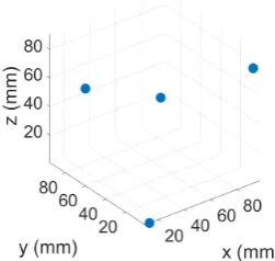
In the following experiments, the optimal DRF was mounted on a milling machine having an accuracy of 0.05 mm to compare measurements of the tracker with a preprogrammed path (Figure 3.1). For evaluating the warming up and different filter settings, the path was programmed within a motion volume of 20 x 10 x 20 cm. The machine stopped for 2 seconds at 27 locations, further denoted as the reference coordinates (Figure 3.1a). Every location in the path was visited three times. For evaluation of the influence of the location of the DRF in the trackers field of view (FOV), reference coordinates in a larger volume (50 x 10 x 50 cm) were used (Figure 3.1b). This time, the machine stopped at 272 positions and each location was visited twice.

In the experiments, the orientation used in Figure 3.1a and 3.1b was used to express the axis. Distance between tracker and the center of the motion volume was 90 cm (z-direction) and 19 cm (y-direction). The actual measurement setup is shown in Figure 3.2. In all experiments, the location of the DRFs was tracked using the optical tracker and data was saved with 120 Hz. No filtering was applied during the acquisition.

Measurement data was imported in Matlab and the measured locations of the DRF were obtained. For each location, 150 data samples were used to calculate the averaged position of the DRF.

3.1.2 Warming up of tracker

For comparing a cold and warmed-up optical tracker, measurements were first per-formed with a cold tracker. The measurement was finished after approximately 7.5 minutes. After warming-up time of 30 minutes was reached, the other experiment was performed. To determine a shift between both measurements, the measured coordinates before and after warming up were subtracted.

To determine a shift in marker location during warming-up time, two DRFs, further denoted as DRF1 and DRF2, were positioned in the center of the FOV of the tracker at a fixed distance of 50 cm. Tracker and DRFs were fixated and did not move during approximately 30 minutes of data acquisition to create a static environment. Data was saved and analyzed to determine whether the measured position of the DRFs shifts during warming up. For better representation of the data, the difference between coordinates of the two DRFs was standardized by:

p_s =p− Pn

i=1pi

(39)

(a)

[image:39.595.118.508.63.473.2]

(b)

Figure 3.1: Measurement setup to test performance the with corresponding axis and dimensions. The optical tracker is shown in red, the reference locations / coordinates in the volume are shown as blue spheres. a) Setup used to investigate the influence on accuracy for warming up and different filter settings. b) Setup used to investigate the influence on accuracy for different DRF locations with respect to the tracker.

[image:39.595.249.376.588.728.2]

(40)

with p being the x-, y- or z-value to be standardized, p_s the standardized x-, y- or z-value and n the number of values in the data p.

3.1.3 Filter settings

The influence of the built-in filters in the optical tracker was tested by performing the same measurements as described in Section 3.1.2, however, with different filtering settings. First, measurements were performed with all filters off. In the second and third condition, position and orientation filters were turned on with values of 0.8 and 1, respectively.

To evaluate the influence of the filters, the trackers’ coordinate system was aligned with the milling machines’ coordinate system using the Procrustes algorithm (Appendix B) [95, 96]. The input in this algorithm was the reference coordinates of the milling machine and the corresponding measurements of the optical tracker. Distance differences between aligned measured coordinates and the reference co-ordinates were calculated to evaluate the performance of the different conditions.

3.1.4 Location of DRF in the field of view

For analyzing the influence of the position of the optimal DRF in the FOV of the tracker, the extended path was used (Figure 3.1b). The distance difference between measured and reference coordinates was calculated as in Section 3.1.3.

Since the measurements were compared to the ground truth, the milling machine, this gave an indication about the trueness of the system. To evaluate the precision, the difference between two measurements at the same location was calculated by subtracting the measured coordinates measured in both rounds.

3.1.5 Statistical analysis

For the experiments with the different filter conditions, it was evaluated whether the measurements were significantly different. The Anderson-Darling test was used with a significance level of 0.05 [104]. If the hypothesis of this test was accepted, the Euclidean distance was assumed to be normally distributed and a paired t-test was used to compare the differences between the conditions [105]. If the hypothesis of the normal distribution for the data was rejected, the Wilcoxon signed rank tests was used to determine whether the found differences in the experiment where significant [106]. These tests were performed using a significance level of 0.05, to reject the hypothesis that the mean Euclidean distances between two experiments is not different.

3.2 Results

3.2.1 Warming up of tracker

(41)

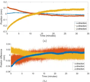
3.2. RESULTS 27 The results from the experiment in the static situation are visualized in Figure 3.3, showing the values of x-, y- and z-coordinates during warming up. The difference between the start and the end of the measurement in the x- and y-direction was 0.02 and 0.14 mm, respectively. The shift in z-direction was larger, with a magnitude of 0.34 mm. The location shift stopped after around 25 minutes. The graph in Figure 3.3a visualizes the jitter generated by the tracker. Jitter in x-, y- and z-direction was 0.01, 0.02 and 0.03 mm, respectively.

(a)

(b)

Figure 3.3: Influence of warming up on performance. a) Both tracker and DRFs were kept in a static position during warming up of the device. A shift of the standardized DRF position is seen in the x-, y- and z-direction. Band-width of the plots show the effect of the jitter. b) Standardized difference between location of DRF1 and DRF2 in all directions.

[image:41.595.162.463.169.441.2]

The shift of both DRFs relative to each other was determined by calculating the difference between the coordinates of both frames. The standardized difference is visualized for the different directions in Figure 3.3b. Shifts of the frames with respect to each other were seen, however, they all were below 0.05 mm.

Table 3.1: Influence of warming-up of the optical tracker on performance. Absolute difference between coordinates measured by a cold and warmed-up optical tracker are reported.

Mean error Max. error

+

− sd (mm) (mm)

X-direction 0.08 +₋0.0352 0.15

Y-direction 0.07 +₋0.0698 0.23

(42)

3.2.2 Filter settings

The results of the filter settings are visualized in Table 3.2 and Appendix C (Figure C.4). The mean Euclidean distance for the situation without filtering was 1.40 mm (sd = 0.66). A filter of 0.8 and 1 resulted in a mean error of 1.39 mm (sd = 0.65) and 1.98 mm (sd = 0.50), respectively.

The Wilcoxon signed rank tests was used as the Euclidean distances of the meas-urements in the experiments were tested to be not normally distributed. No signi-ficant differences were found between applying a filter of 0.8 or no filter (p = 0.207). Significant difference were found between the measurements with no filter or a filter of 0.8 and measurements with a filter of 1 (p < 0.001).

Table 3.2: Influence of different filter settings on tracker performance. Mean and maximal Euclidean distances between measured and reference coordin-ates are reported.

Mean Euclidean Max. Euclidean

distance +₋ sd (mm) distance (mm)

Filter = 0 1.40 +₋0.66 2.35

Filter = 0.8 1.39 +₋0.65 2.38

Filter = 1 1.98 +₋0.50 2.93

3.2.3 Location of DRF in the field of view

To evaluate the trueness of the navigation system in different directions, the track-ers’ measurements were subtracted from the reference coordinates. The mean and highest values for the Euclidean distance and the absolute difference in x-, y- and z-direction are summarized in Table 3.3 and Appendix C (Figure C.5). Mean errors in x- and y-direction were 0.39 mm (sd = 0.30) and 0.39 mm (sd = 0.26), respect-ively, whereas the error in the z-direction was 5.18 mm (sd = 2.44). The maximal reported Euclidean distance was 8.94 mm. The errors seen in this experiment are mainly due to the large inaccuracy in the z-direction, clearly shown in Figure 3.4.

The precision of the system was calculated by subtracting the coordinates from the first and second measurements of all 272 locations (Table 3.3 and Appendix C (Figure C.6). Mean difference was 0.01 mm (sd = 0.01) in the x-direction, 0.02 mm (sd = 0.01) in the y-direction and 0.04 mm (sd = 0.03) in the z-direction. Mean Euclidean distance for the precision was 0.06 mm (sd = 0.03), with a maximal error of 0.32 mm.

3.3 Discussion

(43)

[image:43.595.118.508.290.685.2]

3.3. DISCUSSION 29 Table 3.3: Trueness and precision of the optical tracker, expressed as mean and highest errors.

Trueness Precision

Mean error Max. error Mean error Max. error

+

− sd (mm) (mm) +− sd (mm) (mm)

X-direction 0.39 +₋ 0.30 1.52 0.01 +₋ 0.01 0.08

Y-direction 0.39 +₋ 0.26 0.92 0.02 +₋ 0.01 0.04

Z-direction 5.18 +₋ 2.44 8.93 0.04 +₋ 0.03 0.32

Euclidean distance 5.26 +₋ 2.36 8.94 0.06 +₋ 0.03 0.32

(a)

(b)

Object oriented navigation using augmented reality: a new way of image guided surgery

M.Sc. Thesis Technical medicine