Minimizing expected passenger travel time by optimal buffer allocation in train networks

(1)

1

Faculty of Electrical Engineering,

Mathematics & Computer Science

Minimizing expected passenger

travel time by optimal buffer

allocation in train networks

Henri Pieter Arwyn Goos

M.Sc. Thesis

August 2017

(2)

Abstract

This project considers railway timetable development where the expected passenger travel time is minimized. Buffers are placed in the network to absorb delays and an optimization model is formulated to choose these buffers optimally to minimize expected passenger travel time. A new way of modeling so called ”excess journey time” has been proposed. Given this optimization model, a piecewise-linear approximation of the problem is formulated, where error bounds in terms of the objective function are given. In the model and literature regarding this subject a simplification of reality is made, by dividing the train network into independent parts, to get analytical expressions for the goal function. A model where this simplification is not made is developed and it is found that the simplification causes a severe decrease in solution quality. However, in this research a heuristic is proposed which results in solutions that are very close to optimality. The model is applied to the Dutch intercity network where it is concluded that the model is able to generate timetables meeting the demands necessary for the Dutch network.

(3)

Preface

This report is the result of the graduation project I have been working on for the past couple of months. I really enjoyed the combination of both theoretical mathematical analysis and practical applicability of such an import part every everybody’s life, the railway network. I would like to thank a few people in particular for their help and support during the project.

First of all, I would like to thank Dr. Jasper Goseling for his supervision of the project. I really enjoyed our collaboration and especially that he made me look at the broader mathematical picture at hand, of the sometimes quite practical problems of railway timetabling. Furthermore, he gave the right amount of guidance when needed, while at the same time giving me the oppor-tunity to explore my own ideas.

Next I would like to thank Jo¨el van t Wout for my supervision at NS. He especially gave me insight into the complications, and beauty of railway timetabling problems. Furthermore, he really helped me and gave good advice on the programming implementations of the models devel-oped.

I would like to thank Prof. Dr. Dennis Huisman for allowing me to do my graduation thesis at NS and the guidance he provided during the formulation of the research goals. I would also like to thank the rest of the department PI for their discussions and insights.

Thanks Tjeerd, Leon, Valerie, Manon and Rory for the great time we had as the board of the internship association at NS. The events organized really gave insight into the diverse activities that NS is engaged in. The trip to the Operational Control Center Rail (OCCR) showed me the relevance of this project as the importance of robust, though speedy timetables was strongly em-phasized by OCCR employees. Furthermore, the trip to Frankfurt we organized was an absolute highlight.

Last, thanks to all my friends and family for their support during the time I was working on this project. I hope you enjoy reading this thesis.

(4)

1 Introduction

1.1 Company background

Netherlands Railways (NS) is the largest railway transport provider of The Netherlands. Founded in 1937, as a result of a merge of several different railway providers, NS has operated the entire Dutch network until the 90’s. From then on, a few small providers have made their appearance on mostly small lines. The Dutch railway network is used every day by on average 1.1 million passengers. Next to passenger transport, there is freight train transport, which uses the same infrastructure as passenger trains. I have been doing research at the department PI (Process quality and Innovation). PI is mainly a research department which focuses on developing decision support tools which are being used in other departments of NS. Operations Research is used to give a better understanding and improve decision making in various areas such as Crew Scheduling, Rolling Stock Scheduling and Train Timetabling. In 2008, the department won the Franz Edelman Award for Achievement in Operations Research and the Management Sciences awarded by the Institute for Operations Research and the Management Sciences with their paper, [1] on the use of Operations Research in developing timetables, rolling stock schedules and crew schedules for the Dutch network.

1.2 Planning process and requirements

This section will provide insight in the necessary decisions to be made before a railway network can be taken into operation. In general, there are 5 consecutive phases of decision making when developing a railway system:

1. Passenger Estimation. In order to generate an operating system, it is of great importance to know, or have an estimation of, the amount of passengers traveling from a specific origin to destination. Depending on those numbers decisions can be made about the quality, frequency and size of trains in specific sections. For every Origin-Destination pair, the amount of passengers traveling from that specific Origin to the Destination is estimated, resulting in the so called OD-Matrix.

2. Line Planning. After the OD-matrix is determined, a line plan should be determined. The line plan is the collection of all train lines. Each line has an origin and destination; a frequency and a certain stopping pattern, indicating the stations where the train halts. The line plan problem determines how to cover the railway network with lines best, when considering traffic demand, operating costs and many more.

(8)

4. Rolling Stock Planning. After the timetable is constructed, the next problem is assigning train units to train lines in the timetable. NS owns a lot of different type of rolling stock, for example single deck and double deck trains. For every train line it should be determined which rolling stock is operated. Note that rolling stock does not need to be assigned to a train line for the entire day but can be used on different train lines throughout. Also during peak hours, usually more rolling stock is used compared to off-peak hours. The rolling stock plan describes for every piece of rolling stock when and where it is used throughout the day.

5. Crew Planning. In order to operate the system, drivers and conductors are necessary on trains. There are some challenging aspects that need to be taken into account here. First of all, crew should start and end the day at their home station, as it is undesired that a employee finishes it’s day on the other side of the country. Furthermore, there are some specific demands on the hours of employees. There are constraints on the amount of time an employee is allowed to work uninterrupted. Also a big issue is variation in the work of drivers and conductors. It is undesired by drivers and conductors to work on the same line during the entire day. They want to be employed on a diverse set of train lines. All these factors and many more need to be taken into account when making a crew planning, specifying for every employee on which rolling stock it should be at a specific moment during the day.

The phases described above are executed consecutively. Note however that optimal decision mak-ing in a certain phase is dependent on the decision makmak-ing in a later phase. For example durmak-ing passenger estimation, passenger flows are distributed over the network. But in practice how passengers move is dependent on the timetable, which is determined in a later phase. So the distribution of passenger flows is dependent on the timetable, which is in turn dependent on the passenger flow. In theory all the phases should be executed at the same time. Though there is a lot of research going on on how to integrate these different phases, for example [2], [3], [4], at the moment this is too hard a problem. This report will focus on the timetabling part, assuming the line plan development and passenger estimations have already been performed. The rolling stock and crew planning problem will not be considered.

1.3 Problem motivation

There is a great need to provide fast and quality service for passengers. The railway network is owned by the Dutch government, so the government decides which companies can provide service on which pieces of infrastructure. The NS has the right to continue operating at least until 2025 on the current net. However, the Dutch government has demanded that the NS meets a set of per-formance measures, otherwise they will consider giving other railway companies the opportunity to operate on the net currently used by NS. These performance measures are called KPI’s (Key Performance Indicator), which are among others quality of transfers, transport capacity during rush hour and punctuality.

(9)

the travel time of a passenger is a stochastic variable. By taking the expected travel time as goal function we will take into account both efficiency and robustness, as a trade off is being made by the two in the goal function.

1.4 Research goal

The goal of this research is to develop a way to construct feasible timetables which A) minimize expected travel time and B) can be applied to large networks. There has been previous research, [5], which developed expressions for expected travel time and used this as a goal function to develop train schedules. Here expected travel time was minimized by placing time buffers in the network, allowing to absorb delays occurring during operation. In this research a similar approach will be used where several extensions will be made to meet the specific demands of the Dutch network. Very generally speaking we have the problem of minimizing the expectation of a certain function, where the buffers D are the decision variables. The goal function is dependent on the decision variable D and a set of stochastic variables X, which represents the delays. There are also constraints on the decision variablesD, resulting in a feasible setP. So the problem will be of the following form:

min

D∈PE[f(D, X)].

One of the main considerations when constructing a train schedule is to spread alternative train routes. Different train routes between two stations should be spread out as much as possible to minimize the waiting time until the first mode of transport for passengers arriving randomly at the station. This also gives passengers flexibility to choose their moment of departure. Previous research suggested it is computationally very hard to take this spreading into account. For the Dutch network however, it is of utmost importance for trains to be spread as good as possible. The goal is to examine if there are ways to take into account spreading which is still computationally feasible.

Based on previous research it will most likely be necessary to approximate the goal function by a piecewise linear approximation because of computation time considerations. It is desired that this approximation approximates the original problem as good as possible. We will determine if error bounds between the approximated and original problem, in terms of the goal function values of the solutions found, can be formulated.

Last, in the literature regarding minimizing expected passenger travel time a simplification of the problem is made by dividing the network into independent parts. This will be explained later on in the report. In doing so, analytical expressions for the goal function can be found, which is not possible if this simplification is not made. However, the effect of the simplification on solution quality has not yet been examined in literature. We will develop a model which does not divide the network into independent parts and compare it with the model developed in literature to see if the simplification made is justified.

Summarizing, the main research goals are the following:

1. Develop expressions for the expected passenger travel time depending on the delay charac-teristics of the Dutch network.

2. Construct a new way of modeling the spreading of trains which is numerically applicable to large train networks.

(10)

4. Develop a model which does not divide the network into independent parts to conclude if the simplification made in literature is justified.

1.5 Outline

(11)

2 Literature review

This chapter gives an overview of research already performed on subjects relevant for this project. First, a mathematical formulation of finding timetables will be examined. Then, the distribution of delays based on real life data will be considered. Afterwards research regarding buffer allocation will be discussed. Last, mathematical techniques to solve stochastic programs are examined.

2.1 Train scheduling

Graph representation

We will now focus on how to convert the problem of finding a timetable into a mathematical problem. In order to do so, we will first show how a train network can be represented as a graph, based on for example [6], [5] and in particular for the Dutch network, [7]. Using this graph, a mathematical formulation of the problem will be given.

A train network can be represented by a directed graphG(V, E) whereV is the set of vertices and

Eis the set of edges. The vertices represent stations and the edges represent actions. At a station

i, a trainjhas to arrive and depart. Both are modeled as a vertexV_Arri,j andV_Depi,j . The total vertex

set is the union of all the trains and all the stations it traverses, so V = S i

S j

h

V_Arri,j ∪V_Depi,j i. Furthermore the edges represent interactions between nodes. There are different kind of edges connecting nodes:

1. Ride edge. A trainj can make a ride action, where it is riding from a stationkto stationl. This is modeled as an edge between V_Depk,j andV_Arrl,j .

2. Dwell edge. For every train j, halting at stationi, there is a dwell edge, where the train is waiting to allow passengers to enter the train, between vertices V_Arri,j andV_Depi,j .

3. Transfer edge. This is an action from the viewpoint of the passenger. If a passenger needs to make a transfer at a stationk, transferring from trainito trainj, we construct an edge between the corresponding nodes. An edge will be constructed betweenVarrk,i andV

k,j Dep.

4. Headway edge. A headway edge models the relation between trains who should have a certain minimum headway from eachother for safety considerations. This means that two trains at a certain station should be scheduled a minimum time apart. Commonly, such constraints occur when the trains use the exact same piece of infrastructure. Suppose we have a headway constraint between two trainsiandj at a stationk. These constraints can either be on the arrival part or the departing part. This interaction is modeled as an edge betweenV_Arrk,i and

Vk,j arr orV

k,i Dep andV

k,j Dep.

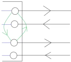
These are all the interactions that happen between nodes. So to represent a network, the graph

(12)

[image:12.595.175.427.106.238.2]

Figure 1: Graph representation of a train network

Here a black edge is a ride activity of a train, a blue edge is a dwell activity of a train and the red edges are passenger transfer actions. The black boxes are train stations. A headway edge looks like the following:

Figure 2: Example of headway edges

Here the two trains use the same piece of infrastructure after leaving the station, so a headway constraint is necessary. The green edges are the headway edges.

Periodic Event Scheduling Problem

The Periodic Event Scheduling Problem (PESP), introduced in [8], deals with finding a feasible solution to an Periodic Event Scheduling Problem, or to conclude that such a solution does not exist. A periodic timetable means that the timetable repeats itself after the timetable period T. So an event taking place at time b, will also take place at time b+nT, withn∈ Z. A periodic

timetable is desired to give passengers more ease to remember the train schedule and get used to it. Usually, a timetable of period T = 60 minutes is desired. From a more general perspective, PESP is a framework to assign time values to periodic events, when there are constraints on the time between specific events. Applied to train scheduling, PESP needs, among others, the graph representation of a train network, described in the previous paragraph. PESP assumes that for every edgee= (i, j)∈E, connecting the verticesiand j, there is a minimum timeleand

maxi-mum timeue allowed for this specific action. PESP answers the following question:

[image:12.595.242.366.338.446.2]

(13)

exist a vectorbsuch that the following holds:

(bj−bi−le) modT ≤ue−le, ∀e= (i, j)∈E.

Note that everybk is the time of a specific node in the graph formulation. So for everyv ∈V = S

i S

j h

V_Arri,j ∪V_Depi,j i a time value bk is assigned, for some k. In essence, PESP is a feasibility

problem. Another way of representing PESP is the following by [6]:

Find (b, n)

s.t. le≤bj−bi+neT ≤ue ∀e= (i, j)∈E

0≤bi< T ∀i∈N

ne∈Z, ∀e= (i, j)∈E

Notice that PESP is a Mixed Integer Linear Program (MILP). A possible extension to the model is to add the constraint that the time an event takes place is a natural number, i.e. bi ∈N ∀i,

as timetables communicated to passengers usually have a precision in minutes. This would make the problem an Integer Linear Program (ILP). By [9] it can be shown that if l, u are integer, and there exists an solution to the problem, then also an integer solution exists to the problem. Furthermore, [9] showed that forT ≥3, PESP is a NP-hard problem, by making a reduction from the k-Vertex Colorability Problem.

In [10] a description of how PESP is solved at NS is given. The solver is called CADANS, which was developed in collaboration with ORTEC, and has several modules. First a solution to the PESP problem is found. In order to do so, a lot of preprocessing is used to remove redundant constraints. After a feasible schedule is found, the next module does post optimization. Event times are moved around such that for example trains driving with a frequency bigger than two are spread as evenly as possible over the cycle period. If no solution is found, CADANS outputs the set of constraints causing the infeasibility and gives suggestions on how to adjust the constraints such that a feasible schedule is possible.

Another recent promising approach is to reformulate PESP as a SAT problem and solve the problem using SAT solvers, described in [11].

2.2 Delay distributions

PESP does not have a goal function. This means any solution is of equal quality in the eyes of PESP. However, in practice this might not be the case. In this research a goal function will be added to the PESP problem. We will develop expressions for the expected travel time and use this as an objective in the model. The travel time of a passenger is a stochastic variable, because there are stochastic delays occurring during operation. To develop expressions for expected travel time, we first need to determine how delays are distributed. There have been several researches on the distribution of delays, which will be analyzed and conclusions about the delay distributions to be used are made.

The research of [12] considers data in the Eindhoven area regarding train delays. An entire week, consisting of 1846 trains were considered. It was concluded that departure delays at stations are best modeled by a negative exponential distribution.

(14)

The Dutch The Hague station was examined by [14]. It was concluded that the Weibull dis-tribution fits the data best, where the shape parameter of the Weibull disdis-tribution tends to be smaller than 1 for arrival and departure actions and bigger than 1 for dwell actions.

Lastly, [15] considered the Indian railway network. Over a period of 30 days, delays were recorded at 26 stations resulting on around 10000 delay recordings. It was concluded that a Weibull distri-bution fits the data best for arrival delays and a log-normal distridistri-bution is best to model departure delays.

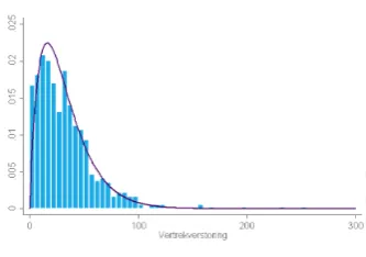
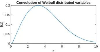
[image:14.595.346.513.355.472.2]

The general trend in the researches seems to be that a Weibull distribution or exponential distri-bution is a good choice for modeling delay distridistri-butions. Since the exponential distridistri-bution is a specific case of the Weibull distribution, it is convenient to consider Weibull distributions. NS also has internal data regarding train delays. The general conclusion was that either an exponential or a gamma distribution were best fits, though it is not clear whether Weibull distributions were also considered. The advantage of using a Weibull distribution comes from the fact that a Weibull distribution is more flexible in terms of the shapes it can take than the exponential distribution. The exponential distribution is a strictly decreasing function, whereas the Weibull distribution is not monotonically increasing or monotonically decreasing. Consider the following figure:

Figure 3: Dataset 1 Figure 4: Dataset 2

These are datasets recorded by the NS at a specific station. For the first dataset an exponential distribution would be a good fit. For the second dataset however an exponential distribution would not be a good fit, as it can not model the increasing trend shown at the beginning of the dataset. A Weibull distribution would be suited to model the second dataset properly. In this research we will consider both exponential and Weibull distributed delays.

Parameter estimation

After deciding the exponential distribution and the Weibull distribution are the distributions to be used in this research, we need to determine a way to estimate distribution parameters, given a set of data. The estimator attempts to approximate the parameters of certain measurements. Various criteria and corresponding algorithms have been developed which all have a different criterium for being a ”good fit”. The most famous techniques are Maximum Likelihood Estimation, Method of Moments and Minimum Squared Error Estimation, as described in for example [16]. Maximum Likelihood Estimation is generally the most used technique. This is the method we will explain here.

[image:14.595.90.516.357.485.2]

(15)

such a way, that the likelihood of the observations that were made is maximal. Suppose there aren independent and identically distributed observationsx1, ..., xn, coming from a distribution

function f(x, θ). Here θ is a vector of parameters. As the samples were independent, the joint density is just the product of the individual density functions. LetL(θ;x1, ..., xn) be the likelihood

function. It follows that the likelihood of doing the observations that we made is the following:

L(θ;x1, ..., xn) =f(x1, ..., xn|θ) = n Y i=1

f(xi|θ).

This function should be maximized with respect to the parameter vectorθto find the maximum likelihood estimator for the observations. Now we will see what this means in practice, when using an exponential and Weibull distribution.

Exponential distribution

Suppose there is a set of delay observationsx1, ..., xn on which an exponential distribution should

be fitted. The exponential distribution hasf(x) =λe−λx_{as distribution function. The likelihood}

function for the exponential distribution is the following:

L(λ;x1, ..., xn) = n Y i=1

λe−λxi ₌_λn_e−λPni=1xi_.

This expressions should be maximized overλi.e. we should solve d

dλL(λ;x1, ..., xn) = 0. Because

ln(x) is a monotonically increasing function, this is equivalent with solving_dλdln(L(λ;x1, ..., xn)) =

0. We get:

d

dλln(L(λ;x1, ..., xn)) = d dλ

h

ln(λn) + lne−λPni=1xii

= d

dλ

"

nln(λ)−λ

n X i=1 xi # = n λ− n X i=1

xi= 0.

This results inλ= n

Pn i=1xi.

Weibull distribution

The Weibull distribution function is f(x) = k_λ x_λk−1

e−(xλ) k

. The likelihood function for the Weibull distribution given the observationsx1, ..., xn is the following:

L(k, λ;x1, ..., xn) = n Y i=1 k λ x_i λ

k−1

e−(xiλ) k

.

To find the best k and λ we should find the maximum of the likelihood function. It is again convenient to take the logarithm of the likelihood function. This results in:

ln(L(k, λ;x1, ..., xn)) = ln

_k λk n + ln n Y i=1

xk_i−1

!

+ ln

n Y i=1

e−(xiλ) k

!

=nln (k)−nkln(λ) + (k−1)

n X i=1

(16)

Now the following system of equation should be solved:

d

dλln(L(k, λ;x1, ..., xn)) =−nk

1

λ+k

n X i=1

xk_i 1

λk+1 = 0

d

dkln(L(k, λ;x1, ..., xn)) = n

k −nln(λ) +

n X i=1

xi− n X i=1

lnxi

λ

ekln(xiλ) _{= 0}

When solving this system of equations, we get by [17] the following expressions forλandk.

k=

"_PN i=1x

k iln(xi) PN

i=1x

k i

− 1

N

N X

i=1

ln(xi) #−1

λ=

"

1

N

N X i=1

xki #k1

Note that the expression forkis not explicit, but can easily be determined with numerical methods such as the Newton-Raphson method [18].

2.3 Buffer allocation

We have seen how train scheduling can be translated into a mathematical problem and how train delays are distributed. The main focus of this research is on buffer allocation. Buffers can be placed in the train network to absorb delays occurring during operation. We will now consider what is already known in literature about buffer allocation in train networks.

The research of [19] considers a train network for which an expression for expected travel time is developed. Depending on the delay distributions, expressions for different kind of actions that passengers can take are developed. The model is applied to a small subnetwork of the Belgian net-work. When comparing the solution of the timetable determined by the model with the timetable in use at that time in the Belgian railway network, a significant improvement was made.

The model of [19] was expanded in [5]. In [19] there were quite some simplifications made on the objective terms. [5] considers the same concept but with less simplifications. A model is devel-oped to determine passenger flows, in order to properly weigh different kind of actions and thus making an analysis of the importance of specific actions/segments. The model is applied to all the Belgium hourly train network and has shown to be able to find feasible solutions, while also taking into account all kinds of safety constraints. A piecewise linearization using two linear segments of the goal function was made.

(17)

2.4 Stochastic Programming

Later on in the report we will have a specific kind of minimization problem, for which the the-oretical groundwork is explained here. The general form of the problem, using the notation of literature used, is minx∈XE[f(x, ξ)] withξ being a stochastic variable. For the problem later on

in the report specifically, an expression for the expectation off is not possible, but f itself is. In this section, literature and techniques useful for solving this kind of problem will be elaborated on.

Stochastic Programming is a framework for modeling optimization problems where uncertainty is involved. Uncertainty can be apparent in different aspects, in the constraints, goal function and there are several criteria possible for when a solution is found. Stochastic Programs can be ”Multi-Stage”, meaning that the solution of the first stage program is dependent on the solution of the second stage problem. The two stage program is most commonly studied in stochastic programming literature, for example in [21] and has the following general form:

min

x∈X c T_x₊

E[f(x, ξ)]

s.t. Ax=b

x≥0

Hereξis random, but follows a known probability distribution. f(x, ξ) again is defined as follows:

f(x, ξ) = min

y q(ξ) T_y

s.t. T(ξ)x+W(ξ)y≤h(ξ)

y≥0

In this formulationx∈Rcan be seen as a first-stage decision variable and y ∈Ras the second

stage decision variable.

For our problem, we do not need to take a second decision based on the realizations ofξ(modeled by the second stage program), just on the expected travel time function. Also, as will be shown when the model for this project is actually developed, there are no constraints on the uncertain realizations ofξ. So for this problem, a first stage problem of the following form is what is desired:

min E[f(x, ξ)]

s.t. Ax=b

x≥0

In the following sections, we will consider two techniques to solve these kind of problems, when

E[f(x, ξ)] can not be analytically determined, but wheref(x, ξ) is known.

2.4.1 Scenario construction

Suppose that the probability distribution of the stochastic vectorξcan be well approximated by a discrete distribution with known probabilitypi for every scenario ξi. Then [22] and [23] write

that the Stochastic Program can be transformed into a equivalent linear program of the following form:

min

N X i=1

pif(x, ξi)

s.t. Ax=b

(18)

This program can be solved by standard methods, as it is just a deterministic program. However, the size of the linear program can become very big very fast. This makes the problem hard to solve numerically. Let the vectorξbe of lengthn. Furthermore, suppose that for every elementξj

in ξwe allow mpossibilities with corresponding probabilities p1, ..., pm. Then the total outcome

space is of sizemn.

2.4.2 Sample Average Approximation

As we saw, we can expect quite some computational issues when we use scenario construction to solve our stochastic program. Sample Average Approximation (SAA) has a similar approach, but does not have the same outcome space problems.

Letx∗ be the optimal solution to our stochastic program, and letz∗be it’s corresponding function value, i.e. z∗ = minx∈XE[f(x, ξ)] =E[f(x∗, ξ)]. SAA approximates the problem by sampling n

samplesξ1_{, ..., ξ}n_{, drawn from the distribution of}_ξ_{. Using these samples an approximation}_x∗

n of

x∗_{and an approximation}_z∗

n ofz∗is sought. These approximations are determined by considering

the following problem:

min 1

n

n X j=1

f(x, ξj)

s.t. Ax=b

x≥0

Herex∗_n is the optimal solution to the above problem andz∗_n is its corresponding objective value, i.e.:

z_n∗ = min

x∈X  

1

n

n X j=1

f(x, ξj)

 =

1

n

n X j=1

f(x∗_n, ξj).

In essence, a Monte-Carlo approximation of the goal function is minimized when using SAA. In the following some properties of SAA regarding bias and convergence ofz_n∗ toz∗ will be shown, by [24].

Bias

It will now be shown whether or not the estimatorzn∗ is biased. z∗nis unbiased ifE(z∗n) =z∗. We

get:

E(z∗n) =E  min

x∈X

1

n

n X j=1

f(x, ξj)

 ≤min

x∈XE  

1

n

n X j=1

f(x, ξj)

 = min

x∈XE[f(x, ξ)] =z.

Here the inequality follows because the minimum of an expectation in bigger than the expectation of the minimum. The estimator is a negatively biased estimator. However, this does not mean that

(19)

Consistency

We knowfn(x∗n)≤fn(x∗), asx∗nis the optimal value when these specificnsamples are considered.

So for n samples, x∗ is not necessarily the optimal solution, but x∗_n is. On the other hand we have _E[f(x∗, ξ)]≤_E[f(x∗_n, ξ)], asx∗ is the optimal solution to the overall problem. Using these inequalities we get:

|z_n∗−z∗|=|fn(x∗n)−E[f(x

∗_{, ξ}_)]_|

= max{fn(x∗n)−E[f(x∗, ξ)],E[f(x∗, ξ)]−fn(x∗n)}

≤max{fn(x∗)−E[f(x∗, ξ)],E[f(x∗n, ξ)]−fn(x∗n)}

≤max{|fn(x∗)−E[f(x∗, ξ)]|,|E[f(x∗n, ξ)]−fn(x∗n)|}

≤ sup

x∈X

|fn(x)−E[f(x, ξ)]|.

Because limn→∞|fn(x)−E[f(x, ξ)]|= 0 with probability one, we get thatz∗nconverges toz∗with

(20)

3 Expected Passenger Travel Time

The following chapter will develop a framework for minimizing expected passenger travel time. The same approach as in [5] is used. However, there are several new contributions. First of all, the expressions developed in [5] and [19] were not very formal, meaning no precise expressions for the stochastic variables were stated. By reasoning and analyzing cases expressions were found. We will give a formal description of the problem. Furthermore, we allow to use Weibull distributed delays as opposed to just exponential delays and give expressions for the goal function. Lastly a new way of modeling excess journey time is developed.

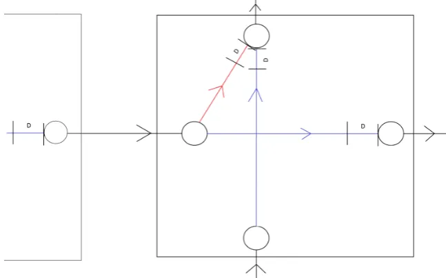
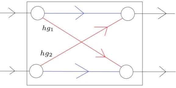
[image:20.595.137.461.402.604.2]

As stated before, buffers are placed in the network to absorb delays. These buffers should not be too small, such that they cannot absorb any practical delay, nor should they be too big, causing passengers to wait unnecessarily long. A trade-off should be made between the two and this is done by considering the expected passenger travel time. Note that the model is not aimed to be robust against any delay. We consider relatively small high frequency delays and not low frequency big delays as a consequence of for example a train having a collision with a pedestrian. High frequency small delays are for example delays as a consequence of leaf on the rail, crowded trains during boarding etc. We allow buffers to be placed after dwell or transfer actions, making them absorb the delay which has occurred starting from the previous buffer in the system. Making the buffers absorb only the delays that have occurred since the last buffer is a simplification, as there might still be delay left in the network not entirely absorbed by the previous buffer. This will be treated in Chapter 5. The following picture shows the idea on a subnetwork at a station:

Figure 5: Example of buffer placement

We use the notation of [5], whereDis the size of the buffer, not to be confused with delay. Delays occur on the black, blue and red edges according to some known distribution function. The big question is what the size of these buffers should be and that is exactly the model we will build to answer this question.

(21)

actions. For these actions, expressions for the expected travel time will be developed, after which the total expression for the travel time of that route can be determined, by simply summing over the travel cost of the actions used. An action consists of all the activities between two buffers that a passenger comes by when traversing the network. The possible actions will now be explained.

First a passenger has to take a departing action to board the train. When the passenger has boarded the train and arrives at the next station, it can either stay in the train, which is a dwell action, or it can make transfer to an other train, which is a transfer action. Every destination can be reached by a finite amount of these actions. Because of the structure of the network and allowed buffer places, an action will always consist of a ride together with a dwell or transfer edge. Depending on the distribution of the delays at these edges and the buffers chosen, we want to know the expected passenger travel time. This will be done for every action possible.

The travel time in practice consists of the minimum travel time, which is the travel time when no delays were to occur, plus the travel time as a consequence of these delays. The first part however is a constant. There are certain minimum travel times for every action, independent from the timetable chosen. We will leave this out of the model, as there is no use in optimizing this. We will focus on minimizing the journey time on top of the technical minimum journey time.

3.1 Action expressions

For every possible action, the expected travel time will be determined in the following parts.

3.1.1 Depart action

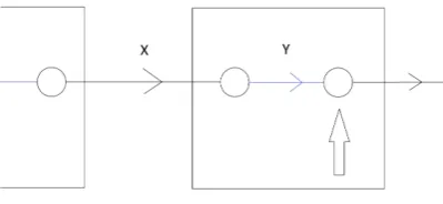
[image:21.595.199.399.492.584.2]

When travelling from an origin to a destination, a passenger first has to depart at the station. Consider the following illustration:

Figure 6: Depart action

Departing passengers arrive at the node the big black arrow is pointing to. After the blue edge, a buffer is placed that can absorb the delays that have occurred since the last buffer, a delayX

during the ride activity and a delayY during the dwell activity. If the cumulative delay is bigger than the buffer, the train will arrive late and the passenger has to wait. In this case, the passenger has to wait for a timeX+Y −D, whereDis the size of the buffer. In case the cumulative delay of the previous part is smaller then the buffer, a departing passenger does not have to wait, as the delay is entirely absorbed by the buffer and thus the train arrives on time. So the stochastic variableCDepart_{, representing the travel time for a depart action, is the following:}

(22)

As we are interested in the expectation, letfDepart _{be defined as}_fDepart ₌

E CDepart(D). By

definition,fDepart is determined as follows:

fDepart=E CDepart(D)

=_E(max{0, X+Y −D})

=

Z ∞

0

Z ∞

0

max{0, x+y−D}fx(x)fy(y)dxdy.

Herefx(x) andfy(y) are the distribution functions ofX andY. As we have seen that delays can

be best modeled by exponential and Weibull distributed variables, we will apply this to the above expression.

Lemma 1. When using an exponential distribution,fDepartis as follows:

fDepart(D) = λx

λy(λx−λy)

e−λyD₋_e−λxD₊ 1 λx

e−λxD₊ 1 λy

e−λxD_.

Proof. See Appendix A.1.1

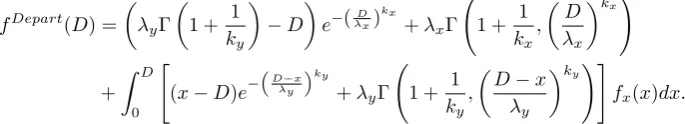
Lemma 2. When using a Weibull distribution,fDepart is as follows:

fDepart(D) =

λyΓ

1 + 1

ky

−D

e−(λxD) kx

+λxΓ 1 +

1

kx

,

_D

λx kx!

+

Z D

0

"

(x−D)e− _D₋_x

λy ky

+λyΓ 1 +

1

ky

,

_D₋_x

λy

ky!#

fx(x)dx.

Theorem 1. For an exponential distribution,fDepart _{is a convex function in}_D

Proof. See Appendix B.1

3.1.2 Dwell action

Suppose that a passenger has already boarded the train and it does not leave or transfer at the next station. So the passenger is using a dwell action. What are the travel costs when a buffer

D is placed for this passenger? In any case, the passenger needs to wait a time D. However, if the cumulative delays occurring during riding X and dwellingY are bigger than this buffer, the passenger needs to wait for an additional time ofX+Y −D. Concluding, the dwell travel time is given by the following stochastic variable:

CDwell(D) =D+ max{0, X+Y −D}.

We are interested in the expectation of this variable, so definefDwell _as_fDwell₌

E CDwell(D).

By taking the expectation, we get the following expression:

fDwell(D) =_E CDwell(D)

=D+E(max{0, X+Y −D})

=D+

Z ∞

0

Z ∞

0

(23)

Lemma 3. When using an exponential distribution,fDepart_{is as follows:}

fDwell(D) =D+ λx

λy(λx−λy)

e−λyD₋_e−λxD₊ 1 λx

e−λxD₊ 1 λy

e−λxD_.

Proof. SincefDwell₍_D_{) =}_D₊_fDepart₍_D_{) and}_fDepart_{was shown above, the result follows}

imme-diately.

Lemma 4. When using a Weibull distribution,fDepart _{is as follows:}

fDwell(D) =D+

λyΓ

1 + 1

ky

−D

e−(λxD) kx

+λxΓ 1 +

1

kx

,

D λx

kx!

+

Z D

0

"

(x−D)e−

D−x λy

ky

+λyΓ 1 +

1

ky

,

_D₋_x

λy

ky!#

fx(x)dx.

Proof. SincefDwell₍_D_{) =}_D₊_fDepart₍_D_{) and}_fDepart_{was shown above, the result follows}

imme-diately.

Theorem 2. For an exponential distribution,fDwell _{is a convex function in} _D

Proof. The sum of two convex functions is convex. Since fDwell₍_D_{) =} _D ₊_fDepart₍_D_{) and}

by Theorem 1, fDepart is a convex function and D is also a convex function, the result follows immediately.

Note that for every buffer placed after a dwell edge, we have anfDepart₍_D_{) function as well as an}

fDwell₍_D_{) function depending on the same buffer}_D_.

3.1.3 Transfer action

Now suppose that a passenger is making a transfer action. For a transfer action, we model expected transfer time as a consequence of the possibility of missing the train the passenger is transferring to. A passenger misses its transfer when he arrives later than the scheduled time of departure of the train it is transferring to. So it is assumed that the train that is being transferred to leaves on time. This is a simplification of reality. If we use this definition, a passenger misses its train if the sum of the delays acquired during the ride and transfer action is bigger than the buffer D. If a passenger misses its train, we assume that a passenger takes the exact same train, but one frequency later. This is a conservative assumption, because there might be other travel routes to the passenger’s destination that make use of other lines, which arrive earlier than the next frequency of the train that is missed. If we let the passenger take the next frequency train, the waiting cost for missing a transfer is _mT , whereT is the timetable period andmthe frequency of the train transferring to. In either case, a passenger needs to wait for a timeD. This gives us the following stochastic variable for the travel time:

CT ransf er(D) =D+1{X+Y > D}T m.

(24)

and taking value 0 ifX+Y ≤D:

1{X+Y > D}=

(

1 ifX+Y > D

0 ifX+Y ≤D

We are interested in taking the expectation. This gives us the following expression forfDepart_:

fT rans(D) =E CT rans(D)

=D+E

1{X+Y > D}T m

=D+

Z ∞

0

Z ∞

0

1{X+Y > D}T

mfx(x)fy(y)dxdy.

Lemma 5. For an exponential distribution,fT rans _{is as follows:}

fT rans=D+ T

m

λye−Dλx−λxe−Dλy

λy−λx

.

Lemma 6. For an Weibull distribution,fT rans_{is as follows:}

fT rans=D+ T

m

Z ∞

0

fx(x)e

−D−x λy

ky

dx+e−(λxD) kx

.

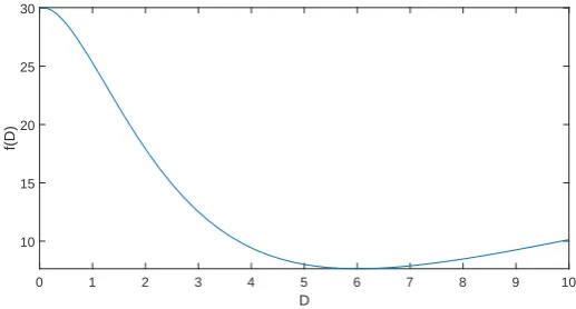
The transfer objective function is not convex, as the following picture illustrates forλx= 1.9 and

λy= 0.6.

0 1 2 3 4 5 6 7 8 9 10 D

10 15 20 25 30

[image:24.595.170.429.498.637.2]

f(D)

Figure 7: Transfer goal function withλx= 1.9 andλy = 0.6

The goal functions of the three actions will be shown and analyzed on their behavior. Forλx= 0.64

(25)

0 5 10 15 20 25 30

D

0 0.5 1 1.5 2 2.5

f(D)

Depart action,λx= 0.64 andλy= 1

0 5 10 15 20 25 30

D

5 10 15 20 25 30

f(D)

Dwell action,λx= 0.64 andλy= 1

0 5 10 15 20 25 30

D

10 15 20 25 30

f(D)

Transfer action,λx= 0.64 andλy= 1

The departure action is a strictly decreasing function. The bigger the buffer, the lower expected travel time for a departing passenger. This is to be expected. A leaving passenger is basically minimizing the expected travel time as a consequence of the train arriving late. A buffer as big as possible is desired to make sure the train is on time. For the parameters used, a buffer bigger than 10 does not have a significant effect anymore, the train is basically guaranteed to arrive on time, so no additional travel time is to be expected.

For a dwell action, the graph is a strictly increasing function, so a buffer as small as possible is desirable. A passenger already in a train has no advantage of buffer placement. Introducing buffers only increases the probability that the train has to wait unnecessary, for example when the previous delays are smaller than the buffer. This is why for a dwelling passenger, a buffer of zero is optimal.

For a transfer action, we see the function has an obvious minimum. If the buffer chosen is too small, the train to which the passenger is traveling to will most likely be missed. When the buffer is chosen too big, the transfer to the next train will almost certainly never be missed, however the passenger does need to wait for an unnecessary long time. The optimal solution is somewhere in between.

As was stated before, for every buffer placed after a dwell edge, both thefDepartand thefDwell

(26)

0 5 10 15 20 25 30 D

5 10 15 20 25 30

fDep

(D)+f

Dwell

[image:26.595.191.408.111.236.2]

(D)

Figure 11: fDepart+fDwell

3.2 Excess journey time

The objective functions developed in the previous sections described the travel time of a passenger starting from the moment that the train the passenger takes should arrive, until the passenger leaves the network. This objective function, however, does not describe the time a passenger waits for its transport when the passenger arrives randomly at the station. Those are passengers that arrive at the station independently of the actual train timetable. Think for example of passengers who go the the station immediately after their last appointment at work is done, which might be any time. The time that passengers have to wait until the scheduled moment of their first form of transport is called excess journey time. This excess journey time will be added to the objective function. By adding this to the objective function, as a result, alternative routes between origin destination pairs will be more spread in time. Of course not every passenger arrives randomly or independent of the timetable. For a certain fraction of passengers, the excess journey time will be added.

We do enforce that trains with a frequency bigger than 1 in the timetable period T are spread perfectly. Meaning that if a train has a frequency m >1, then the inter arrival times of those trains are enforced to be _mT . This is because of customer clarity. By adding the objective function described above we will spread trains of different series as good as possible.

Previous research, [5], has also researched adding the excess journey time to the objective function. Although expressions for the excess journey time are easy to achieve, the numerical implementa-tion got quite problematic, as massive computaimplementa-tion times prohibited soluimplementa-tions with a satisfacimplementa-tional optimality gap. This was caused by the unknown order of trains during scheduling, to be explained in the following sections, where a lot of constraints had to be added to model this unknown order.

In this section first we will derive expressions for the excess journey time. Afterwards, we will discuss how the problem was modeled in the research of [5]. Last we will introduce a new way of taking into account excess journey time, which is expected to have better computation time.

3.2.1 Deriving excess journey time expressions

We are interested in finding the expected waiting time when a passenger arrives randomly at the station. The expression for excess journey time has been well documented in the literature. In the literature however a stochastic inter arrival time is assumed with known distribution function. For our case the interarrival times are not stochastic as we are considering the time betweenplanned

(27)

in literature where stochastic inter arrival times are assumed, and our approach where inter ar-rival times are deterministic. First we will derive the expected waiting time when considering the deterministic arrival times, afterwards we will derive the way shown in literature and show how the two are connected.

Suppose we have a set of N trains serving the same origin and destination. Suppose that these trains are scheduled at timesb1, ..., bN, withbi≤bi+1∀iand 0≤bi≤T ∀i. Now definesias the

inter arrival time between bi and bi+1, so si =bi+1−bi ∀i= 1...N −1 and sN =b0−bN +T.

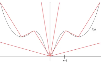
Given these headway times, the waiting time when arriving at a timet, 0≤t≤T is characterized by a sawtooth functionY(t). The following figure expresses this:

Figure 12: Sawtooth functionY(t) characterizing excess journey time

In this example, the interarrival times are 20, 10 and 30 minutes respectively. The sawtooth functionY(t) states for a giventthe waiting time if a passenger were to arrive at timet. Letf(t) be the distribution function of the arrival time of a passenger. Then the expected waiting time is given as_E(w) =RT

0 Y(t)f(t)dt. We assume that passengers arrive uniformly over the interval,

so we have f(t) = _T1 as distribution function. The expected waiting time now is given by the

following expression: E(w) = RT

0 Y(t)dt

T . Letsi be the distance between the zero’s of the sawtooth

function. Naturally, the sum of interarrival times sum up toT. This gives us the following:

E(w) =

RT

0 Y(t)dt

T =

PN i=1

1 2s

2

i

T =

1 2T

N X i=1

s2_i.

This is the expression that we are going to add in the objective function, for every OD pair where multiple transportation possibilities are possible. Now we will take a look at how expected waiting time is determined in the literature, for example [25]. The general approach is to get an expression for_E(w) using the following:

E(w) =Expected total passenger waiting time per vehicle departure

Expected passengers per vehicle departure .

It is assumed that the interarrival times between two consecutive forms of transport is stochastic with a distribution functiong(h). Furthermore letn(h) be the amount of passengers arriving in a headway of lengthhand letw(h) be the mean waiting time for passengers arriving in a headway of lengthh. ThenE(w) can be expressed in the following way:

E(w) =

R∞

0 n(h)w(h)g(h)dh

R∞

0 n(h)g(h)dh

(28)

Let the arrival rate of passengers be λ, then n(h) = λh. Furthermore, the mean waiting time when arriving in a headway of lengthhis w(h) = h₂, if uniform arrival of passengers is assumed. Plugging in these expressions we get:

E(w) =

R∞

0 λ

h2

2g(h)dh

R∞

0 λhg(h)dh

= 1 2

R∞

0 h

2_g₍_h₎_dh

R∞

0 hg(h)dh

=1 2

E(h2) E(h)

.

Note that this expression is the same as the expected residual service time in an M/G/1 queue. Also an analogy with the limit of the expectation of residual life in a renewal process can be made. The headway times in our model basically are a sequence of numbers, of which, according to the above, we want the second and first moment. Let the second moment of [s1, ..., sN] be defined as

1

N PN

i=1s 2

i and the first moment as N1 PN

i=1si. Then we get the following:

E(w) =

1 2

1

N PN

i=1s 2

i

1

N PN

i=1si

.

Because we knowPN_i₌₁si =T, we getE(w)21T PN

i=1s 2

i, which is exactly the same expression as

already determined before.

The problem with implementing the expressions developed above is the yet unknown order of trains during optimization. The si used in the goal function are determined by taking the time

difference between two consecutive trains. However, since a timetable is still being constructed, it is unknown which trains are consecutive trains at the station considered. As a consequence, it is unclear how the si used in the goal function should be defined. This is the core of the problem.

First the modeling of the unknown order problem in [5] will be explained, afterwards a new way of modeling the unknown order of trains is introduced.

3.2.2 Modeling in previous research

Consider a randomly arriving passenger at a station and suppose there areN possible trains the passenger can take in the cycle period to get to its destination. Letb1, ..., bN be the time of arrival

of trains 1, .., N. In order to determine the subsequent order of b1, ..., bN , which are not yet

ordered, a new set of variables ˆbi, using the same values as bi are introduced. Here the modulo

T values of the starting times, such that 0≤ bi ≤ T, are taken. To enforce ordering, ˆbi ≤ˆbi+1

is added as a constraint. Since the values used in ˆbi are the same as in bi, a permutation matrix

p ∈ _NN×N _{is introduced to enforce the increasing order. This is done by adding the following}

constraints:

∀i:

               ˆ

bi ≤ˆbi+1

ˆ

bi =PN_j₌₁pijbj

pij ∈ {0,1} ∀j

PN

j=1pij = 1

PN

j=1pji = 1

Now that ˆbi is of increasing order,si can be determined as follows:

si= ˆbi+1−ˆbi i= 1...N −1

sN = ˆbN −ˆb1+T

Furthermore, because the termspijbjare nonlinear, as bothpij andbj are undetermined variables,

(29)

ˆ_b_i ₌PN

j=1pijbj in the constraints is replaced by ˆbi = PN

j=1hij, where the following constraints

onhij are added:

−T(1−pij)≤hij−bj≤T(1−pij)

0≤hij ≤T pij

Using these constraints has the effect thathij =pijbj ∀i, j. So ifpij = 0 thenhij= 0 and likewise

ifpij = 1 thenhij=bj. However we now only use linear constraints.

As we can see a lot of constraints and binary variables have to be introduced to model the unknown order of trains. This is one of the reasons of the significant increase in computation time. The way of modeling is summarized below:

min 1 2T

N X i=1

s2_i

s.t. ˆbi≤ˆbi+1 ∀i= 1, ..., N

0≤bi ≤T ∀i= 1, ..., N

pi,j∈ {0,1} ∀i= 1, ..., N, j = 1, ..., N

N X j=1

pi,j= 1 ∀i= 1, ..., N

N X j=1

pj,i= 1 ∀i= 1, ..., N

ˆ_b

i= N X j=1

hij ∀i= 1, ..., N

si= ˆbi+1−ˆbi ∀i= 1, ..., N

−T(1−pij)≤hij−bj≤T(1−pij) ∀i= 1, ..., N, j = 1, ..., N

0≤hij ≤T pij ∀i= 1, ..., N, j = 1, ..., N

3.2.3 New way of modeling

After taking a considerate look at the modeling of excess journey time in [5], the main problem is expected to be caused by introducing the permutation matrix p. If there are N trains, N2

binary variables have to be introduced. Furthermore, if N trains are considered, 2N constraints on the binary variables introduced in the permutation matrix have to be introduced to make sure that the sum over the rows and columns equals 1, makingpan actual permutation matrix. Lastly, for every elementpij , linearization constraints have to be added to linearize the expression

ˆ_b_i ₌PN

j=1pijbj. For everypij , four constraints are needed, resulting in 4N2 binary constraints.

So in total 4N2+ 2N binary constraints are needed. As can be seen, even for relatively low N, already a lot of extra variables and constraints have to be introduced. This is probably the main cause of the excessive computation times in [5].

The newly proposed method uses the so called cyclic order of trains. [6] defines the cyclic or-der of a set of trains as the following:

Definition 1. The events 1,...,k, scheduled at timesb1, ..., bk are said to be cyclically sequenced

in the order 1→...→kif:

(30)

By considering the cyclic order of trains, we take the periodic nature of the timetable into account. For example, in a cyclic timetable, the order of trains 1,2,3 is exactly the same as the order 2,3,1 and 3,1,2 because the timetable repeats itself. The cyclic order basically stores all these possible equivalent orders into 1 order, namely the cyclic order 1→2→3.

We will now take a look at the amount of cyclic orders possible when there are N trains. This will be necessary in the new way of modeling the unknown order of trains.

Theorem 3. If there areN trains, then there are (N−1)! cyclic orders of trains.

Proof. Proof by induction.

Basis. Suppose we have two trains, then the sequence 1,2 is obviously equivalent with the se-quence 2,1, leaving 1 cyclic order. So the base case holds.

Induction step. Assume the induction hypothesis holds for N = k, i.e. k trains have (k−1)! different cyclic orders. Now we have to show thatk+ 1 trains can be scheduled ink! ways. Con-sider thektrains, which can be scheduled in (k−1)! ways. Now we have to determine in how many ways we can add the lastk+ 1thtrain. Thek+ 1thtrain can be placed before the 1st,2nd, ..., kth

train and after the kth train. Leaving us k+ 1 possibilities. However, since placing the train before the 1st _{train is equivalent with placing the train after the} _kth _{train, we actually have} _k

possibilities to place the last train. In total we have (k−1)!k=k! possibilities, as was to be shown.

It can be concluded by induction that N trains can be scheduled in (N −1)! different cyclic orders.

The new way of modeling is based on the observation that if there areN trains, we basically have to choose between (N−1)! cyclic orders. When a cyclic order is chosen, this determines how the

siused in the goal function are determined. Our decision problem will now consist of which order,

out of the (N−1)! possibilities is chosen. We introduce (N−1)! binary variablesw1, ..., w(N−1)!,

where every binary variable indicates whether or not that specific cyclic order is chosen. As we should select exactly 1 order, we have the following constraint:

(N−1)!

X i=1

wi= 1, withwi∈ {0,1} ∀i.

Now that a specific order of trains is enforced, we should make sure that the correct inter-arrival times are used in the goal function for the chosen order. Let the vectorgi represent the beginning

times of the trains chosen in the ith _{order. So} _gi ₌ _{_b

1i, ..., bNi}. For example, when 3 trains

need to be spreaded, according to theorem 3, there are 2 cyclic orders, namely the cyclic order 1 → 2 → 3 and the cyclic order 1 → 3 → 2. For this example we get g1 ₌ _{_b

1, b2, b3} and

g2 ₌ _{_b

1, b3, b2}. Now the interarrival times between trains for order i is the time difference

betweenbi

j+1 and bij ∀j. However, because the interarrival times are of course between 0 and T,

the modulo of the time difference betweenbi_j₊₁andbi_j is taken by definingg_j,ji ₊₁=bi+1−bi+nT

withnan integer and 0≤gi

j,j+1≤T. So just like in the previous research a modulo operation is

needed. Lets1, ..., sN be the variables used in the objective function. If the ithorder of trains is

chosen, thesj should be equal to the order chosen ingi. Sos1=gi1,2, ..., sj=gj,ji +1, ..., sN =gN,i 1.

(31)

following constraints:

(N−1)!

X i=1

wi= 1, wi∈ {0,1},∀i

(sk−gk,ki +1)wi= 0 k= 1...N, i= 1, ...,(N−1)!

By multiplying the expression (sk −gik,k+1) with wi we make sure that only in case order i is

chosen the variables sk used in the goal function are determined by the order i, so the other

possible orders have no influence in this case. We now have introduced (N−1)! binary variables and (N−1)!N binary constraints. To give a better understanding, an example will be treated below.

Example 1. Suppose we need to spread 3 trains. Then according to Theorem 3, there are 2 cyclic orders of these trains, namely the order 1→2→3 and the order 1→3→2. Letw1be the binary

variable indicating whether or not cyclic order 1 → 2 → 3 is chosen and let w2 indicate if the

cyclic order 1→3→2 is chosen. Nowgi _{is the following:} _g1₌_{_b

1, b2, b3} andg2={b1, b3, b2}.

It follows thatgi

j,j+1 is as follows:

g₁1_,₂=b2−b1+n1T g21,2=b3−b1+n4T

g₂1_,₃=b3−b2+n2T g21,2=b2−b3+n5T

g31,1=b1−b3+n3T g21,2=b1−b2+n6T

The constraints used are the following:

w1+w2= 1

(s1−g11,2)w1= 0 (s1−g21,2)w2= 0

(s2−g12,3)w1= 0 (s2−g22,3)w2= 0

(s3−g13,1)w1= 0 (s3−g23,1)w2= 0

Note that ifw1= 1, the values ofsiwill be chosen according to the cyclic orderg1and ifw2= 1,

the values ofsi will be chosen according to the cyclic orderg2.

Note that in the expression above, (sk−gik,k+1)wiare nonlinear terms, as undetermined variables

are multiplied. A linearization technique is used to replace these nonlinear terms by linear terms, by adding extra constraints.

To do so we are going to introduce a variable zk,i. The goal is to replace the nonlinear

con-straint (sk−gik,k+1)wi= 0 byzk,i = 0. However,zk,i should of course take the exact same values

as (sk−gik,k+1)wi. This is enforced by adding the following constraints:

LB·wi≤zk,i≤U B·wi

(si−gk,ki +1)−U B(1−wi)≤zk,i≤(si−gk,ki +1) + (1−wi)LB

Here U B and LBare upper and lower bounds of (sk−gk,ki +1)wi. As both we have 0≤sk ≤T

and 0≤gi

(32)

constraints enforce that if wi = 1, then zk,i = sk−gk,ki +1. On the other hand if wi = 0, then

zk,i= 0.

The goal function and their constraints now look like the following, if we have to spreadN trains:

min 1 2T

N X

i=1

s2_i

s.t.

(N−1)!

X i=1

wi = 1,

wi∈ {0,1} i= 1, ...,(N−1)!

zk,i= 0, k= 1, ..., N, i= 1, ...,(N−1)!

−T wi≤zk,i≤T wi k= 1, ..., N, i= 1, ...,(N−1)!

(si−gk,ki +1)−T(1−wi)≤zk,i≤(si−gk,ki +1)−T(1−wi) k= 1, ..., N, i= 1, ...,(N−1)!

0≤gi_j,j₊₁≤T j= 1, ..., N, i= 1, ...,(N−1)!

g_j,ji ₊₁=bi_j₊₁−b_ji+nT j= 1, ..., N, i= 1, ...,(N−1)!

For both models integer variables are needed to make sure the expressions are modulo T, so between 0 and T, using the same amount of constraints. The amount of binary variables and constraints needed in both models will now be compared, as the amount of binary variables and constraints are expected to have the most significant influence on computation time compared to continuous variables. As was shown before, the model of [5] needs to introduceN2_{binary variables}

and 4N2_{+ 2}_N _{binary constraints. The newly proposed model needs (}_N ₋_{1)! binary variables}

to consider the possible cyclic orders. (N−1)!N =N! constraints are needed to make sure the right interarrival times is chosen, corresponding to the chosen order of trains. Every one of these constraints is linearized, using 4 inequality constraints, resulting in 4N! constraints. 1 additional constraint is necessary to make sure that exactly 1 order is chosen. This results in the following table:

N = 2 N = 3 N = 4

Sels Variables=N2 4 9 16

Constraints=4N2_{+ 2}_N ₂₀ ₄₂ ₇₂

Arwyn Variables=(N−1)! 1 2 6 Constraints=4N! +1 9 25 97

Table 1: Amount of binary variables and constraints for both models

(33)

3.3 Objective

Now all expressions needed for the goal function have been derived, so the total goal function can be composed. First an expression for the expected travel time without excess journey time will be explained. Afterwards the excess journey time will be added. Every passenger traverses a certain route when traveling from his origin to destination. Every routes consists of a set of consecutive actions, described in the previous section. The total travel time is the sum of the travel time on these actions. Let a routetbe a set of actions, sot={t1, ..., tn}, where everytiis a dwell, transfer

or depart action. For a passenger following a routet, its expected travel time is:

E Rt=

|t|

X i=1

fti₍_D

ti).

Here |t| is the size of the vector t, so the amount of actions needed for route t. Suppose that an amount opwt follow a route t. Then the total cost of routet iswt multiplied by the above

expression. Furthermore, we want to consider all possible routes and sum over them. LetRT be the set of all possible routes. This results in the following expression for the Total TraveltimeT T:

E(T T) =

X t∈RT

wtE Rt=

X t∈T

|t|

X i=1

wtfti(Dti).

The excess journey time has not been incorporated in the expression forT T yet. LetSP be the total set of train pairs that should be spreaded where an elementp= ([p1, ..., pN], wp)∈SP is a

tuple storing the specific trains,p1, ..., pN that should be spreaded and the amount of passengers

using these trains, wp. Furthermore, we assume a fraction a, 0≤a≤1, of all passengers arrive

randomly, so for these passengers the excess journey time should be added to the goal function. A fraction 1−aof the passengers adjust their arrival time at the station according to the timetable, so no excess journey time should be modeled for these passengers. We get the following:

E(T T) =

X t∈RT

|t|

X i=1

wtfti(Dti) +a

X p∈SP

pN

X i=1

wp

1 2Ts

2

i.

3.4 Constraints

Several constraints need to be taken into account to get an operational feasible schedule. In order to do so, we need to get expressions for the time that every event, or node in the graph formula-tion, takes place. Depending on the buffersD chosen, expressions for the time of the events can be determined. The constraints necessary to guarantee an operational feasible schedule are with regards to those event times.

Let us first consider edges regarding train activities. The length, or time, of an edge connect-ing two events or nodes, is the time difference between these events. Every edge or activity has a minimum timeme, for example the technical minimum time that is necessary for a train to travel

between two consecutive stations. On top that, for a dwell edge, there is a buffer De. Letbe be

the starting time of edgeeand leteebe the ending time of edgee. Then the following constraints

are added to the model:

∀e∈ERide: be+me=ee

∀e∈EDwell: be+me+De=ee.

Suppose we have an edge e1 and an edge e2, for which the ending node of e1 is the same as