Master thesis
Routing and scheduling of the parking
enforcement in Amsterdam
Author: Jan Groeneveld
ARS | Traffic & Transport Technology
Supervisor: D.G. Speekenbrink
University of Twente
Supervisor: Dr. Ir. J.M.J. Schutten
Supervisor: Dr. Ir. M.R.K. Mes
Management summary
In December 2016, Egis Parking Services B.V. (EPS), who was hired by the municipality of Amsterdam to manage the parking enforcement within Amsterdam, tasked ARS T&TT (ARS) with the development of a planning tool that supports their work. The Smart Parking unit of ARS started to work on this project and additionally, requested a separate research on how such a planning tool can be developed. From February 2017 until September 2017, we conducted this research.
The idea behind the parking enforcement is that more parking visitors pay the parking fee. Whenever a parking visitor in Amsterdam wants to pay the parking fee, the visitor has to register the license plate of his/her car. The license plate is uploaded to a database afterwards. The on-street agents of EPS visit different neighborhoods of Amsterdam, i.e., they drive through neighborhood in parking enforcement vehicles (PEVs) and scan parked cars in different neighborhoods. During this process, the license plates of the parked cars are uploaded to a different database. By comparing both databases, it can be determined whether a visitor, whose car was scanned by a PEV, paid the parking fee. If a visitor did not pay, a penalty charge notice (PCN) is generated. For some exceptional cases, it is required that another agent who follows the PEVs on a scooter (PEF) checks the parked car on-site.
The output of our routing algorithm is a schedule of all neighborhood visits for all PEVs. In order to do this in a smart manner, we have to consider EPS’ objective. The municipality of Amsterdam measures EPS’ performance regarding the parking enforcement based on two Key Performance Indicators (KPIs): the payment rate, which is the ratio between paying visitors and all visitors, and the control chance, which is the probability that a non-paying visitor receives a PCN. From the control chance target, we can derive the number of PCNs that is needed in order to meet the control chance target. This number is called the PCN target, which we use instead of the control chance. Concerning the evaluation of EPS’ performance, it is important that every neighborhood belongs to one of 10 KPI areas. Within one KPI period, which lasts three months, EPS has to meet certain targets of the KPI that are determined by the municipality. The municipality of Amsterdam takes random samples of neighborhoods and examines the payment rate. Whenever the payment rate measured by the municipality is below the pre-set target, the PCN target is considered. The rationale behind this is that EPS cannot directly influence the payment behavior of the visitors and therefore they have to show that their effort of fining the non-payers is at least high enough. If both targets are below the pre-set targets, then the KPI area is in a malus state and EPS will receive a fine. If in all KPI areas at least one of the targets is met, then EPS receives a bonus for those KPI areas where the payment rate exceeds the pre-set target. Apart from the KPI targets, EPS tries to visit every neighborhood once a week. Therefore, we derive the following three priorities in the following order:
1. Meet either the payment rate target or the PCN target of every KPI area.
2. Maximize the control chance in chosen KPI areas in order to eventually increase the payment rate and maximize the performance bonus.
3. Visit every neighborhood once a week.
Finally, it is required that our routing algorithm does not only maximize the number of PCNs but also takes these priorities into account. For that reason, we do not only consider the expected number of PCNs that can be obtained by visiting a neighborhood but also the neighborhood’s Target Factor and Visit Day Factor, which take the mentioned priorities into account. Since the routing algorithm requires inputs, we first have to compute:
Travel times (the travel time from one neighborhood to another)
Service Times (the time that is needed to scan a neighborhood)
Number of PCNs (the expected number of PCNs by visiting a neighborhood)
Margin of error (an increase of the KPI targets to account for uncertainty)
For predicting the number of PCNs, we concluded that it is required to know the following ratios:
The occupancy ratio, which is the ratio between occupied parking spots and all parking spots in a neighborhood at a given time
The PCN ratio, which is the ratio between PCNs and all scans in a neighborhood at a given time This PCN ratio can also be split into the visitor ratio, which is the ratio of visitor scans (scanned cars that belongs to paying or non-paying visitors) and all scans, and the non-paying ratio, which is the ratio of all non-paying visitor scans (PCNs) and all visitor scans. Our prediction model (or forecasting method) is based on an estimation of this occupancy ratio and a neural-network based prediction for the PCN ratio. Multiplying the number of parking spots with the occupancy ratio and the PCN ratio results in our forecast of the number of PCNs. This research also contains an extensive data analysis of the PCN ratio. We observed in our data analysis that:
The PCN ratio depends on the weekday
The PCN ratio does not depend on the weather
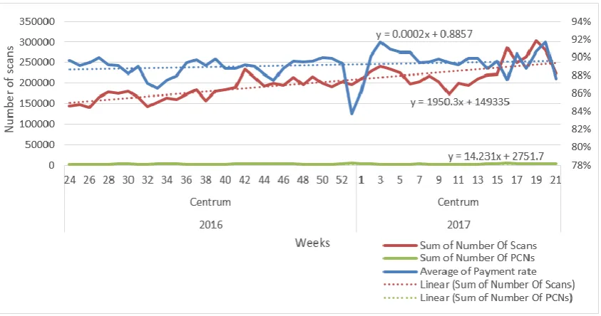
The payment rate increased from approximately 89% to 90% within one year (1.6.2016-1.6.2017) The routing algorithm that we present in this research, first creates a solution based on a greedy algorithm and then tries to optimize this solution by constructing new solutions based on an ant colonization optimization (ACO) algorithm. Since it is possible to visit one neighborhood multiple times a day, one ingredient of our greedy algorithm is very important, namely the stability function. Our proposed stability function accounts for the fact that when the PEVs goes to a neighborhood that has been visited already the same day, it is possible that some non-paying visitors from the earlier visit are still in that neighborhood. Even though we show that the ACO algorithm performs well for one vehicle, it had difficulties to find better solutions than the greedy algorithm when 12 vehicles are deployed, which is the standard number of vehicles used by EPS (from Monday to Saturday). Finally, we perform a sensitivity analysis, a simulation study, and compare our prediction model and routing algorithm to the ones currently used at ARS. We prove that our neural network has a more accurate prediction (+4%) regarding the PCN ratio and that our routing algorithm leads to better results (+34%) than the current implementation of ARS algorithm when the same inputs are used (assuming that our stability function is correct). We are confident that our planning tool improves the current situation at EPS by automating the planning process, increasing the number of obtained PCNs, and faster reaching the KPI targets. This will finally lead to less fines and more rewards. Furthermore, we have shown that our greedy algorithm can create a planning for 90 days within 6 hours.
Preface
With this thesis, I am not only finishing my master program but also my entire study period at the University of Twente. On the one hand that makes me sad because I am closing a great period of my life, during which I have learned a lot about the world of industrial engineering, lived in three different countries, and I have met and worked with very special people. On the other hand, I am happy that I succeeded, I am proud to present my master thesis and I am looking forward to the future.
I thank ARS T&TT and Rolf Appel for the opportunity and giving me such an interesting project. Even though I never expected that one day I would optimize parking enforcement, I really liked the technical challenges that came with it. In this regard I also thank Ahmad Al Hanbali, who supervised my bachelor thesis and helped me finding this project.
My special thanks go to my supervisor Dennis Speekenbrink at ARS T&TT, who made always time for feedback and discussions despite of his busy agenda. It was a pleasure working with you and your critical thoughts and feedback were most helpful.
Of course, I also owe a great deal of thanks to my supervisors Marco and Martijn. You both spent a lot of time in proof-reading and finding every grammatical, writing, or essential error and answered my emails in no time. After hearing about other students’ experiences, I know that this should not be taken for granted.
Definitions & Notations
: An optimization technique that is inspired by the pheromone trails that ants leave, in order to attract other ants to the ways that used to work well in the past.
The company where the research is conducted and which provides traffic and transport technology solutions to businesses and government.
The middle point of a neighborhood based on the scans of 3 months.
An arc routing problem in which the route of a postman that has to deliver mail to different streets is optimized.
The average number of PCNs within a not-paid-for parking hour, which is estimated. : A pre-set target regarding the control chance that is determined by the municipality for one KPI area regarding one KPI period.
The company that is responsible for most of the operational aspects of on-street fiscal parking in Amsterdam, such as on-on-street parking meter enforcement.
A type of performance measurement that evaluates the success of an organization or of a particular activity.
A recurring period of three months within which the KPI targets must be met. The 10 different areas in Amsterdam that are measured.
Include the PCN target, which is derived from the control chance target, and payment rate target.
A small geographical unit within a KPI area.
The ratio between non-paying visitors and all visitors in a neighborhood at a given time.
In this thesis we limit the parking enforcement to the activities related to the on-street parking meters in Amsterdam.
The ratio between the occupied parking spots and all parking spots in a neighborhood at a given time.
A scooter that is driven by a parking enforcement follow-up agent that go to the parked cars that need further investigation and/or where a PCN must be issued locally.
A vehicle that is driven by a parking enforcement agent and that scans parked cars.
Indicates the time interval of a certain region (independent from KPI area and neighborhood) during which visitors have to pay for parking.
The ratio between paying visitors and all visitors in a neighborhood at a given time. : The performance of the payment rate in a KPI area, which is measured by dividing the current payment rate by the payment rate target.
A pre-set target regarding the payment rate that is determined by the municipality for one KPI area regarding one KPI period.
A parking fine that is issued whenever a non-paying parking visitor is detected.
The performance of the number of PCNs in a KPI area, which is measured by dividing the current number of PCNs by the PCN target.
The ratio between non-paying visitor scans and all scans in a neighborhood at a given time. A target that is derived from the control chance target. Indicates the number of PCNs that has to be achieved in a KPI within a KPI period.
Parking enforcement agent who drives the PEV. Parking enforcement agent who drives the PEF.
The time needed to scan a certain neighborhood.
A parameter that determines how important the KPI areas get after they have reached one of the KPI targets.
: A parameter that restricts the travel distance between two scheduled neighborhoods.
The time needed to travel from the center point of a neighborhood to the center point of another neighborhood.
A parameter that reduces the accounted travel time when the PEV leaves a break location.
A parameter that restricts the travel time between two scheduled neighborhoods.
A problem in which a salesman has to travel to a certain set of cities and the travelled distance has to be minimized by choosing the best sequence of visits.
The ratio between visitor scans and all scans in a neighborhood at a given time. A scan of car that belongs to a paying or non-paying visitor.
The same problem as the TSP but usually with multiple vehicles. A database that contains all important payment parking information. A bonus that increases when the payment rate target is exceed. The bonus is only given when the control chance and the payment rate target are met.
A parameter that determines the fraction non-paying visitors that stay at a visited neighborhood for a certain amount of time.
A parameter that determines whether a swap is performed.
1 Introduction ... 1
1.1 Context ... 1
1.2 Problem identification ... 3
1.3 Research scope ... 4
1.4 Problem approach ... 4
2 Current situation ... 6
2.1 Routing ... 6
2.2 Planning ... 11
2.3 Conclusion ... 12
3 Literature ... 13
3.1 Problem review ... 13
3.2 Routing heuristics ... 15
3.3 Input models ... 19
3.4 Conclusion ... 23
4 Computation of inputs... 25
4.1 Challenges of the historical data ... 25
4.2 Margin of error ... 25
4.3 PCN prediction ... 27
4.4 Travel times ... 47
4.5 Service times ... 48
4.6 Conclusion ... 48
5 Routing algorithm ... 49
5.1 Planning horizon... 49
5.2 Notation ... 49
5.3 Objective function ... 50
5.4 Routing algorithm ... 55
5.5 Conclusion ... 63
6 Results ... 64
6.1 Design of experiment ... 64
6.2 Prediction models ... 65
6.3 Sensitivity analysis ... 66
6.4 Simulation study ... 74
6.5 Improvement of current situation ... 76
6.6 Conclusion ... 77
7 Conclusion and Recommendations ... 78
7.1 Contribution to the literature ... 78
7.2 Practical conclusion ... 79
8 References ... 82
1 This project is part of the Master program Industrial Engineering and Management at the University of Twente. It has a limited time span of 6 months. We conduct this research at the Smart Parking business unit of ARS Traffic & Transport Technology. Within this research, we develop a planning tool to support the parking enforcement activities that concern the on-street parking in Amsterdam. In this thesis, we denote these activities as parking enforcement.
This first chapter provides an introduction to this research. Section 1.1 introduces the stakeholders who are involved in this project and describes core activities associated with parking enforcement. In Section 1.2, we identify the problem this research addresses. Finally, we define the scope of this research in Section 1.3 and explain our approach to tackle this problem including our research questions in Section 1.4.
In order to better understand the background of this research, this section describes the stakeholders involved in the parking enforcement and how the parking enforcement in Amsterdam is executed and how its performance is currently measured.
In this research project about the parking enforcement in Amsterdam, there are three important stakeholders: the municipality of Amsterdam, ARS Traffic & Transport Technology (ARS), and Egis Parking Services B.V. (EPS).
ARS is a company in The Hague that provides traffic and transport technology solutions to business and governments. Since 1997 it is active in its home market, the Netherlands, but also internationally (ARS T&TT, 2017). Concerning on-street parking, ARS is a partner in a joint venture with Egis Project, called Egis Parking Services B.V. (EPS). EPS operates from the shared service center in Amsterdam. In January 2016, the municipality of Amsterdam hired EPS to manage all operational aspects of on-street fiscal parking, such as for permit management, ticket machine maintenance, and parking enforcement. In December 2016, EPS tasked ARS with developing a planning tool regarding the parking enforcement in Amsterdam.
Amsterdam has over 140,000 on-street parking spaces, dispersed amongst 10 fiscal parking areas. Each of these areas is divided into neighborhoods. In total there are 538 neighborhoods with different sizes (see Figure 1) of which 320 have fiscal (paid) parking.
2 Every visitor who travels to Amsterdam by
car and parks in a fiscal parking space has to pay a parking fee. The fee depends on the time the vehicle remains in the parking space and the parking space itself. A visitor can pay the parking fee through several electronic systems, such as parking meters, mobile payment, call-payment, and online visitor registration. The payment information of these systems, including the vehicle’s license plate, is uploaded to a “Parking Rights Database” (PRDB).
Parking enforcement vehicles (see Figure 2) drive through the neighborhoods, scan parked cars in the fiscal parking space, and take pictures of these. We further denote
these vehicles as PEVs and their driver as PEV drivers. While scanning, the license plates of the parked cars are uploaded to a central system, which stores the recognized license plates. By comparing both databases, it can be determined which visitors did not pay a parking fee so that a Penalty Charge Notice (PCN) can be issued. The amount of the PCN is the sum of a fixed amount (the penalty) and one hour of the parking fee that should have been paid for that parking spot. In general, parked cars as scanned by the PEV can be classified as:
Parking permit holders
Exceptions
Visitors
o Paying visitors
o Non-paying visitors
Domestic
International
o Unclear situation Parked cars with a parking permit belong to inhabitants that pay on a long-term basis. Some vehicles are exempted from parking payment because they are considered as exceptions (e.g., loading/ unloading vehicles and emergency vehicles). For this research, the most important groups are the domestic and international visitors who did not pay for their parking and visitors whose situation is unclear at first sight. Domestic non-paying visitors receive a
PCN that is issued
automatically. This automatic process is not possible for international non-paying visitors.
That is why an off-street agent will contact a follow-up parking enforcement agent who drives with a scooter to the location of the international car to issue a PCN on-site (see Figure 3). As for the PEV, in this research, we denote the scooters as PEFs and their drivers as PEF drivers. For some vehicles, it is unclear if they paid for their parking. Possible reasons are that the license plate is unreadable in the provided images or it is unclear whether there is a loading/unloading process. Since it has to be determined whether the vehicle belongs to a visitor that did not pay, these unclear parking situations require an on-site visit of the PEF driver as well. At this moment, there is a 1-to-1 relation between the PEVs and PEFs, i.e., one PEF follows one PEV. If a visitor receives a second PCN and did not pay the first one, the municipality may request that a wheel clamp is placed on the vehicle.
Figure 2 – Parking enforcement vehicle
3 The purpose of parking enforcement is to ensure that citizens and visitors pay for their parking. The municipality of Amsterdam measures this by means of a Key Performance Indicator (KPI), namely the “payment rate”. The payment rate is the willingness of visitors (non-permit holders) to pay for their parking. In other words, it is the ratio of paying visitors in relations to the total number of visitors. In this research, we denote it as the payment rate and not payment ratio because this is the term that is currently used at ARS. The municipality measures the payment rate in all 10 fiscal parking areas for a period of 3 months by taking random samples. In this research, we denote these areas as KPI areas and the 3 month period as the KPI period. The performance of EPS with regards to the parking enforcement is evaluated by the payment rate that the municipality measures for every KPI in a KPI period. Unfortunately, there is no direct relationship between the parking enforcement and the payment rate because it is unknown to what extent the parking enforcement affects the payment rate. In theory, it could happen that EPS does a great job and every visitor who does not pay a parking fee gets a PCN but the payment rate does not increase. Even though, this is very unlikely because the general assumption is that people pay for parking if the chance of getting a fine is too high. This assumption, that enforcement influences the payment rate, is confirmed in the literature, as Adiv and Wang (1987) show that parking non-compliance level increases as the level of enforcement decreases. Peliot (2004) indicates that this phenomenon can be described as a relational economic choice (portfolio choice), i.e., the driver asses the risk of getting a fine and the amount of the fine versus the regular parking costs. This theory is confirmed by Adiv and Wang (1987) and Elliot and Wright (1982) in an empirical study. Since it is not desirable for the municipality to increase the amount of the PCNs or the parking fee, they want to increase the risk of getting a fine (PCN). For that reason, the municipality does not only consider the payment rate but also the “control chance”, which is the probability that non-paying visitors receive a PCN. Only if the payment rate is not met, the municipality will consider the control chance as a means to establish that “enough” effort has been put into enforcement. Only when for all KPI areas either the payment rate or control chance target has been achieved, the municipality will give EPS a performance bonus for any KPI area where the payment rate exceeds the pre-set target (not for the control chance). Note that every KPI area has different targets for the payment rate and control chance. These targets increase after every KPI period (up to certain maximum values).
In this section, we define the problem which enables us to formulate an approach to tackle the problem. In the context of this thesis, EPS has two planning tasks, namely the daily routing of the PEVs and the staff scheduling. Currently, EPS handles both planning tasks manually. Since capacity is limited and enforcement targets are rising, there is a need for an automated planning tool that delivers the following three outputs:
PEV routing: The planning of the daily PEV routes indicates at which time drivers need to be in a certain neighborhood. Obviously, this will require inputs to determine realistic and smart routes.
Staff scheduling: The staff has to be assigned to the vehicles. This can be done separately from the PEV routing.
Estimation of the KPI results: An indication to what extent the KPI targets will be met at the end of the KPI period. This supports the decision process with regards to the needed capacity for the short term.
The goal of this planning tool is to increase the efficiency of the available capacity and reducing the effort of manual scheduling. Increasing efficiency is always linked to an objective. As we derive from Section 1.1.3, it is the objective to meet either the targets of the payment rate or the control chance in all KPI areas. Furthermore, EPS wants to visits every neighborhood once a week. In fact, EPS has an order of priority with regards to their targets:
1. Meet either the payment rate target or the control chance target of every KPI area.
2. Maximize the control chance in chosen KPI areas in order to eventually increase the payment rate and maximize the performance bonus.
3. Visit every neighborhood once a week.
4 ARS has started the development of such a planning tool in December 2016. This thesis, which started in February 2017, can be seen as a part of this project that aims to develop a more accurate and smarter planning tool that is supported by scientific literature.
In this section, we discuss which aspects we do and do not consider in this project. The objective of this graduation project is to create a planning tool for the parking enforcement in Amsterdam. In Section 1.2, we stated that the planning tool should deliver the PEV routing, the staff scheduling, and an estimation of the KPI results. The staff scheduling, however, is an independent smaller and less crucial problem and therefore we only focus on the development of a routing algorithm that determines the daily routing of the PEVs and also estimates the KPI results. The development of this planning tool involves three main steps:
First, before creating any outputs, we need inputs for the routing algorithm. To this end, we have to analyze which inputs are needed. For example, we need to know how long it takes to travel between the neighborhoods and how long it takes to scan one. Furthermore, we need to know how many PCNs we expect to generate when scanning a neighborhood. For the development of these inputs, we can make use of the literature, the knowledge of EPS, and data of all parked cars that were scanned since January of 2016.
Second, we develop the routing algorithm. This routing determines for every PEV the sequence of neighborhood visits (including the time). The routing algorithm implies also embedding this algorithm in a programming platform. EPS requires that the total computational time must not exceed a daily limit of six hours. Apart from the routing, the routing algorithm needs to estimate whether the KPI targets will be met at the end of the KPI period.
Third, the planning tool needs to be validated afterwards, such that the functionality and contribution of the tool can be proven.
Consequently, the planning tool consists of useable input data and a routing algorithm that is embedded in an application. In this regard, there are some related aspects that are beyond the scope of this research. First of all, we only assign drivers to neighborhoods and not to streets. Even though we do have data of all scans since January of 2016 including GPS coordinates, EPS asks for a system that is based on neighborhoods. The reason behind it is that a street based planning is too strict and cannot be executed accurately it practice. A neighborhood routing gives EPS more flexibility. Additionally, creating street-based routes would increase the solution space of the problem and therefore the computation time. Furthermore, we do not consider decisions made on an online operational level, i.e., we do not take dynamic aspects into account. For instance, if an accident occurs, the original route is not adjusted. Such online changes require detailed real-time instructions (e.g., a navigation tool in the car) but this is currently not possible. Neither, do we make decisions on a strategic level such as reducing the number of PEVs. Nevertheless, the capacity might change in the future and therefore we use number of deployed PEVs as a parameter. Furthermore, we do not consider reducing the number of PEFs and assigning them to multiple PEVs because we focus on the routing of the PEVs. Moreover, we do not consider the fact that visible presence of the PEV possibly prevents parking violations (comparable with the presence of police cars preventing possible crimes).
This section describes the plan of approach of this research, which also includes the research questions. Before introducing all research questions, we present our research goal, as concluded in Section 1.2:
“Develop a planning tool for the parking enforcement that maximizes the number of PCNs in such a way that the required KPI targets are met in all KPI areas and eventually a payment rate bonus is achieved”
From this research goal, we derive research questions, which are discussed in the following chapters: Chapter 2 – Current situation
This chapter describes the current situation of the planning and routing. By conducting interviews and reviewing the available data, we answer the following two questions:
How does the current routing of the PEVs look like?
5 Chapter 3 – Literature
This chapter introduces the required literature of this thesis. First of all, we want to know if this problem or similar ones have been introduced to the literature and how these problems have been tackled and solved. Furthermore, we investigate how inputs for the routing algorithm can be developed by using available data. Furthermore, we are interested in theories about the parking and payment behavior of visitors. Consequently, we answer the following questions:
What is known in the literature about problems regarding the routing of parking enforcement or similar routing problems?
o Which solution methods does the literature suggest?
What is known in the literature about the parking and payment behavior?
What is known in the literature about developing input data?
o What is known about travel times or speed models?
o What is known about prediction models?
For the purpose of this literature research, we use Scopus and Google Scholar. Chapter 4 – Computation of inputs
This chapter analyzes the gathered data and investigates patterns and statistical characteristics in order to compute inputs that can be used for the routing algorithm. We answer the following questions:
How can we use the historical data to develop inputs for the routing algorithm?
In order to answer these questions, we first clean the available data and make some transformations if necessary. Afterwards, we analyze the data to find patterns and develop a data model. By means of this data model, we create inputs for the planning tool.
Chapter 5 - Routing algorithm
Within this chapter, we design a routing algorithm that can be embedded in the planning tool. Furthermore, we discuss the choices with regards to the algorithm and the strategies behind it.
What kind of algorithm is most suitable for this problem?
How can we measure the performance of the algorithm? Chapter 6 - Results
In this chapter, we analyze the results of the planning tool to make sure that this tool is actually working and improving the current situation.
To what extent is the proposed planning tool improving the current situation? Chapter 7 – Conclusion and Recommendations
6 This chapter describes the current situation of the routing (Section 2.1) and planning process (Section 2.2) at EPS. This chapter is based on interviews with the manager and drivers from EPS and data that they provided.
In this section, we describe the routing of the PEVs in terms of different routing characteristics proposed by Van der Heijden and Van der Wegen (2011). These general characteristics are applicable to every routing problem.
The fleet consists of a certain number of homogenous PEVs and PEFs, which is set a priori. Currently, one PEF is assigned to one PEV and 12 of both are used in the daily operations. A vehicle can be unavailable due to maintenance or other reasons. Every morning the vehicles are refuelled.
[image:13.595.73.512.396.632.2]The fleet of PEVs and PEFs starts and finishes the daily routes at the same depot. In between, the drivers have breaks, which are further explained in Section 2.1.5. For these breaks, the fleet may return to the depot or to two extra break locations, which are exclusively used for breaks. The fleet must take every break at one of the three possible break locations. The break locations are scheduled based on the shortest extra travel time with regards to the scheduled route. Figure 4 shows all neighborhoods, the depot (marked in red), and the two break points (marked in green).
Figure 4 – Overview of neighborhoods, the depot, and the two break locations
7 about factors influencing the number of visitors and the payment behavior. The data analysis of these factors is part of Chapter 4. This analysis helps us to make predictions about how many PCNs we can expect when scanning a neighborhood. The time that a PEV driver needs to scan a neighborhood, is denoted as the service time. The service time depends on the average speed of the PEV and the length of the route within the neighborhood. The PEV drivers indicate that these service times are time-dependent due to traffic congestion. Chapter 4 deals with estimation of this service time and the prediction of the expected PCNs while scanning. Since it is possible to go more than once a day to one neighborhood but it is not possible to issue multiple PCNs on one day for the same vehicle, another problem arises, namely: How many PCNs can we expect the second time? Or more correctly: How many non-paying visitors remain on the parking spot until the next visit? This problem is discussed further in Section 4.3.4.
Regarding the locations of the neighborhoods, the neighborhoods have the shape of polygons and ARS has the GPS coordinates of polygons’ edge points. The sizes, shapes, and number of corner points are different for every neighborhood. ARS created an extra GPS coordinate for every neighborhood that is the center point of all scans during 3 months and therefore we denote this point as center point.
As for the service time, the travel times between two neighborhoods depend on the distance between the neighborhoods and the average speeds of the PEV.
The speed is influenced by time-dependent traffic congestion. Note that we do not consider the allowed speeds of the streets since we do not consider streets in this research. Moreover, due to one-way streets or one-way traffic congestions, the speeds might be directed, i.e., it matters if the PEV goes from neighborhood i to j or from j to i. Chapters 4 discusses whether it is necessary and possible to include this.
The distance between two neighborhoods depends on the last scanned street of the previous scheduled neighborhood and the first scanned street of the following neighborhood. ARS created a distance matrix using the center point of every neighborhood that we explained in Section 2.1.3. This distance matrix considers the actual distance traveling through all streets from one center point to another. This leads to a problem because the center point lies within the neighborhood. Therefore, this distance includes also the distance between the point when the PEV enters or leaves the scheduled neighborhood and its center point. Consequently, if we measure the distance between the two centers points of the two neighborhoods, we will calculate twice the redundant distance from the entry/exit point of the neighborhood and its center point. This distance, however, is difficult to determine as it depends on the last scanned street of the previous neighborhood and the first scanned street of the following neighborhood. Chapter 4 further discusses this problem and the development of useful travel time input. Furthermore, we must not forget that the PEV keeps scanning parked cars while traveling to other neighborhoods. For instance, the PEV travels through other neighborhoods to get to the next destined neighborhood. However, in that case, the PEV drivers mostly use through-streets that are less dense with regards to the number of PCNs. In Chapter 4, we also answer the question whether it is useful to include this phenomenon.
In order to create proper routes, we have to take several time restrictions due to shifts, breaks and parking regimes into account. Regarding the shifts, there are three regular shifts from every day of the week:
Regular shifts (from Monday until Sunday):
Day shift: 8.00-16.30
Evening shift: 15.30-23.40
Night shift: 23.30-4.00
However, there is also on additional shift on Sundays due to different parking regimes: Additional shift (on Sundays):
Sunday afternoon shift: 11.30-20.00
Even though on Sundays there are additional Sunday afternoon shifts, the total number of deployed PEVs is usually less on Sundays than during the week.
8 the PEV driver must not have a visit that starts before 16.00 and finishes after 16.15. The shift change from evening to night shift is done at the depot, hence we do not have to take it into account. Except for the night shift, all shifts including one 20-minute break and one 35-minute break. The night shift drives without a break. EPS decided to vary break times a bit in order to spread the breaks around and to avoid moments in which no PEV is driving around. The reason behind this is that it lead to visitors not paying during break times of the PEV drivers. Currently, this is done by means of the vehicle number, where even numbers have one break regime, and uneven numbers have another. The break times are as follows: Even numbers:
Dayshift breaks: 11.30 – 12:05 and 13.45 – 14.05
Evening shift breaks: 18.15 – 18.50 and 21.15 – 21.35
Sunday afternoon shift breaks: 14.15 – 14:35 and 17.00 – 17.35 Uneven numbers:
Dayshift breaks: 11.15 – 11.50 and 14.00 – 14.20
Evening shift breaks: 17.45 – 18.20 and 20.45 – 21:05
Sunday afternoon shift breaks: 14.00 – 14.20 and 16.45 – 17.20
Even though EPS uses fixed break times, we can use a tolerance of 15 minutes to increase the flexibility of the planning. The PEV driver should choose the break location which leads to the shortest total travel time. The PEF drivers have to do the follow-up work. Correspondingly they go to the same break location and their breaks start a bit later than the ones of the PEV drivers.
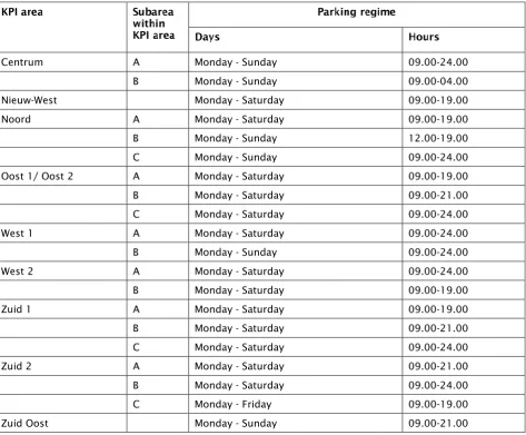
Furthermore, there are different parking regime times, which indicate at which time a visitor has to pay a parking fee. The parking regimes times of Amsterdam can be seen in Table 1.
Centrum A Monday - Sunday 09.00-24.00
B Monday - Sunday 09.00-04.00
Nieuw-West Monday - Saturday 09.00-19.00
Noord A Monday - Saturday 09.00-19.00
B Monday - Sunday 12.00-19.00
C Monday - Sunday 09.00-24.00
Oost 1/ Oost 2 A Monday - Saturday 09.00-19.00
B Monday - Saturday 09.00-21.00
C Monday - Saturday 09.00-24.00
West 1 A Monday - Saturday 09.00-24.00
B Monday - Sunday 09.00-24.00
West 2 A Monday - Saturday 09.00-24.00
B Monday - Saturday 09.00-19.00
Zuid 1 A Monday - Saturday 09.00-19.00
B Monday - Saturday 09.00-21.00
C Monday - Saturday 09.00-24.00
Zuid 2 A Monday - Saturday 09.00-21.00
B Monday - Saturday 09.00-24.00
C Monday - Friday 09.00-19.00
[image:15.595.71.545.346.737.2]Zuid Oost Monday - Sunday 09.00-21.00
9 Sometimes the parking regime times differ within one KPI area. Therefore, some of them are split into two or three subareas. ARS already assigned the neighborhoods to different parking regimes.
We do not have restrictions with regards to the length of the route. The route is only restricted by the time as mentioned before.
Cost factors are factors that need to be minimized. In a usual VRP, this would be the travel times or travel distances. As we further explain in Section 2.1.8, the maximization of the number of PCNs is the crucial output in this routing problem. Even though EPS has no interest in minimizing the travel distances, it is important that the travel distances are reasonable such that the PEF driver can still follow the PEV on the scooter. A smart maximization of the number of PCNs will automatically minimize travel times to some extent to improve the efficiency of the route. Nevertheless, it could be interesting to keep track of the travel distances for two reasons. First, the routes will not have the same amount of kilometers. So assuming all PEV are interchangeable, at a later time it may make sense to arrange vehicles amongst schedules such that they do not all reach their next maintenance requirement at the same time. Second, if we assume that some vehicles have less range than others (e.g., electric vehicles) it may be useful to assign specific vehicles to routes with less travel distance. Therefore, the travel distance would be nice to have but should not impact the core of the routing algorithm.
As already mentioned in Section 1.2 the most important KPI for the municipality is the payment rate, the fraction of visitors that pay for parking. The problem of this KPI is that we do not have the information of all visitors. The number of paying visitors is known as they are saved in the PRDB. Logically, the non-paying visitors are not registered in the PRDB. Only those non-non-paying visitors are known that are scanned and issued with a PCN but these are not all of them. Basically, the payment rate (p) should be measured with the following formula:
p =
𝑁𝑢𝑚𝑏𝑒𝑟 𝑜𝑓 𝑝𝑎𝑦𝑖𝑛𝑔 𝑣𝑖𝑠𝑖𝑡𝑜𝑟𝑠𝑁𝑢𝑚𝑏𝑒𝑟 𝑜𝑓 𝑝𝑎𝑦𝑖𝑛𝑔 𝑣𝑖𝑠𝑖𝑡𝑜𝑟𝑠 + 𝑁𝑢𝑚𝑏𝑒𝑟 𝑜𝑓 𝑛𝑜𝑛 𝑝𝑎𝑦𝑖𝑛𝑔 𝑣𝑖𝑠𝑖𝑡𝑜𝑟𝑠
,
but since we do not know the number of non-paying visitors, it is measured with the following formula:
p =
𝑁𝑢𝑚𝑏𝑒𝑟 𝑜𝑓 𝑠𝑐𝑎𝑛𝑛𝑒𝑑 𝑝𝑎𝑦𝑖𝑛𝑔 𝑣𝑖𝑠𝑖𝑡𝑜𝑟𝑠𝑁𝑢𝑚𝑏𝑒𝑟 𝑜𝑓 𝑠𝑐𝑎𝑛𝑛𝑒𝑑 𝑣𝑖𝑠𝑖𝑡𝑜𝑟𝑠
.
Therefore, we can only estimate the payment rate for a certain sample of scans. For example, a PEV starts to scan a small neighborhood with 100 parking spots at time t = 0. After 10 minutes at t = 10, the PEV has scanned all 90 cars. Out of these 90 cars, 40 cars had a parking permit and 50 cars were visitors. 10 of these visitors, did not pay the parking fee and will receive a PCN. Assuming that nobody left a parking spot or arrived to the parking spot within these 10 minutes, we can make the following conclusions from this example:
The occupancy ratio is 90%, which is the ratio between occupied parking spaces and the total number of parking spaces
The visitor ratio is 50/90%, which is the ratio between visitor scans (all scanned cars that belong to a paying or non-paying visitors) and all scans
The non-paying ratio is (40/50%), which is the ratio between non-paying visitors and all visitors (equal to 1-p)
10 Figure 5 – Pyramid showing the factors on the number of PCNs
Regarding the number of PCNs, approximately 10% of the PCNs that are immediately generated are removed afterwards. A common reason for this is that a visitor pays the parking fee but registers the wrong license plate and therefore receives a PCN. After a complaint, these PCNs will be deleted and therefore not accounted with regards to the KPI targets. Within this research, we only consider the number correctly issued PCNs.
As stated in Section 1.2, EPS tries to increase the control chance in order to eventually increase the payment rate and show the municipality that the enforcement effort is at least high enough. The control chance is supposed to indicate the fraction of non-paying visitors that are “caught” and issued a PCN. However, the municipality, and consequently also EPS, computes the control chance (c) by dividing the number of correctly issued PCNs in a KPI area by the estimated number of not-paid-for visitor parking hours. Consequently, this means that the control chance is not a probability. More accurately, we should call it the average number of PCNs per not-paid-for visitor parking hour. This could be improved by dividing the number of not-paid-for visitor hours by the average parking duration of non-paying visitors. However, since this is the way the performance is measured by the municipality and EPS, we continue explaining how this number is estimated. For this purpose, the municipality uses the payment rate (p). First, they estimate the total number of visitor parking hours by dividing the paid-for visitor parking hours, which can be retrieved from the PRDB, by the payment rate:
Visitor parking hours =
𝑝𝑎𝑖𝑑 𝑓𝑜𝑟 𝑣𝑖𝑠𝑖𝑡𝑜𝑟 𝑝𝑎𝑟𝑘𝑖𝑛𝑔 ℎ𝑜𝑢𝑟𝑠𝑝
.
In order to estimate the number of not-paid-for parking hours, they subtract the paid-for visitor parking hours from the total number of visitor parking hours:
𝑛𝑜𝑡 𝑝𝑎𝑖𝑑 𝑓𝑜𝑟 𝑣𝑖𝑠𝑖𝑡𝑜𝑟 𝑝𝑎𝑟𝑘𝑖𝑛𝑔 ℎ𝑜𝑢𝑟𝑠 =
𝑝𝑎𝑖𝑑 𝑓𝑜𝑟 𝑣𝑖𝑠𝑖𝑡𝑜𝑟 𝑝𝑎𝑟𝑘𝑖𝑛𝑔 ℎ𝑜𝑢𝑟𝑠
𝑝
− 𝑝𝑎𝑖𝑑 𝑓𝑜𝑟 𝑣𝑖𝑠𝑖𝑡𝑜𝑟 𝑝𝑎𝑟𝑘𝑖𝑛𝑔 ℎ𝑜𝑢𝑟𝑠 =
(
1𝑝
− 1) ∗ 𝑝𝑎𝑖𝑑 𝑓𝑜𝑟 𝑣𝑖𝑠𝑖𝑡𝑜𝑟 𝑝𝑎𝑟𝑘𝑖𝑛𝑔 ℎ𝑜𝑢𝑟𝑠 .
Finally, the formula of the control chance (c) is:
c =
𝑁𝑢𝑚𝑏𝑒𝑟 𝑜𝑓 𝑃𝐶𝑁𝑠(1
𝑝−1) ∗ 𝑝𝑎𝑖𝑑 𝑓𝑜𝑟 𝑣𝑖𝑠𝑖𝑡𝑜𝑟 𝑝𝑎𝑟𝑘𝑖𝑛𝑔 ℎ𝑜𝑢𝑟𝑠
.
The measured payment rate, the control chance target (𝑐𝑡𝑎𝑟𝑔𝑒𝑡), and the paid-for visitor parking hours can
be inserted in the formula. By doing so, the number of PCNs needed in every KPI area for the 3 month of the KPI period can be estimated. This number is called the PCN target:
Number of
PCNs
Number of visitors
Number of scans
11
PCN target = c
target∗ (
1p
− 1) ∗ paid for visitor parking hours.
Since the PCN target is always derived from the control chance target, we always refer to the PCN target and the payment rate whenever we speak about KPI targets further in this research.
There is one major problem with regards to the KPI targets, namely the fluctuation of the payment rate and the paid-for visitor parking hours. Both can be estimated but a false estimation can lead to not achieving the PCN target. Every KPI period, the municipality measures the payment rate by taking random samples to check whether the target is reached. The size of the samples and when and where they are taken is unknown. Consequently, EPS has the problem that they do not know which payment rate the municipality finally uses to measure their performance. This makes it difficult to set a fixed PCN target. The good thing is that EPS can estimate the payment rate based on a large number of recent scans, namely all scans of their daily planned routes. As the daily planned routes are not planned randomly, one can say that they use non-random samples but with large sample sizes to represent the entire population of the KPI areas. The paid-for visitor parking hours are based on historic data saved in the PRDB. We will tackle the uncertainty problem of the payment rate and the paid-for visitor hours in Chapter 4.
Considering the KPI targets, a KPI area can have one of the three following statuses:
Malus – None of the targets is reached. In this case there is a fine for the difference between the control chance target and the actual performance since the effort of EPS is not big enough.
Neutral – The PCN target is reached and the payment rate measured by the municipality does not exceed the
Bonus – The payment rate measured by the municipality exceeds the payment rate target.
Note that EPS only receives a bonus for a KPI area if none of the KPI areas has a malus status. In this regard, it is important to remember that due to the uncertainty of the KPI targets it is possible that they turn out to be lower than expected at the end of the KPI period (further discussed in Chapter 4). Finally, as already mentioned in Section 1.2, the objective of the routing follows a certain order of priority:
1. Meet either the payment rate target or the PCN target (respectively the control chance) of every KPI area (bring all KPI areas at least to a neutral status).
2. Maximize the PCN target in chosen KPI areas in order to eventually increase the payment rate and maximize the performance bonus.
3. Visit every neighborhood once a week.
The order of these priorities must not be interpreted as a sequence of actions, i.e., first we only act on the first priority, then on the second, and finally on the third. All priorities should rather be taken into account at all times. Even though the third point of the priority list (“visit every neighborhood once a week”) is only a soft constraint, it is important to visit all neighborhoods in order to collect data. Otherwise, the following scenario might happen:
KPI area A consists of 5 neighborhoods A1, A2, A3, A4, and A5. The daily measured payment rate of KPI area A is below the required payment target. Consequently, the PEVs have to scan this area to reach the PCN target. If the PEV drivers know that it is likely that they can issue a lot of PCNs in the neighborhoods A1 and A2, they will probably drive there, in order to reach the PCN target faster. If they keep doing this, they create blind spots because they do not scan neighborhoods A3, A4, and A5 anymore. Hence, they do not collect data of the payment rate in these neighborhoods. These blind spots are dangerous since they lead to a misconception of average payment rate of the entire KPI area. If the municipality measures the payment rate only in one of these “blind spot neighborhoods” (A3, A4, A5), it might happen that the payment rate that is measured by the municipality is actually lower than expected. Considering the formula of the PCN target, this target increases with a lower payment rate. In the end, this could lead to EPS not meeting neither of the KPI targets.
In this section, we briefly explain how EPS currently manages the planning of the PEV routes.
EPS determines the staff scheduling for one year. Normally, they deploy around 12 PEVs from Monday to Saturday and less on Sundays. For one shift with 12 PEVs, they usually need 28 people: 12 driving the PEVs, 12 driving the PEFs, and 4 operating as off-street agents. For the night shift, EPS usually schedules only one PEV. If they know that there will be a shortage of drivers in the next two week, they can hire extra drivers from an external company.
12 hours there have been in the previous week (Tuesday till Monday) every Tuesday. As described in Section 2.1.8, they use all this recent data to estimate both KPI targets of the current KPI period. EPS adjusts the PCN targets every day such that they know many PCNs they should have issued until the day of the planning. For instance, if they estimated that the PCN target of KPI area A is 900 at the end of the KPI period, which is day 90, then they would have required 400 if today was day 40. This means that they assume in this planning that every day they can issue the same number of PCNs. Every day, they plan the routes for the next day as follows:
1. The results of the past two days are analyzed.
2. They check whether all drivers are available for the next day. Reasons for not being available are holidays, illness, or appointments.
3. The availability of the PEVs and PEFs is checked. Sometimes they are unavailable due to maintenance or damage.
4. They determine the routes by assigning the PEV drivers to certain neighborhoods that they should visit between the breaks. The routes are based on the analysis of the last days, the results of the KPI targets, and their priority order as discussed in Section 2.1.8.
Even though the planning is done one day in advance, it can still happen that employees are suddenly unavailable the following day. In this case, employees who were initially scheduled to operate as an off-street agent need to drive a PEV, to ensure that the capacity of the PEVs is efficiently used.
We conclude from the current situation that there are several inputs needed for routing algorithm.
KPI targets: Every 3 months the fixed KPI targets for the payment rate and control chance (respectively PCN target) are changed. The PCN target is recomputed every day to ensure that it contains the most recent data.
Available capacity: In this project, the capacity depends on the availability of PEVs, PEFs, and shifts. On the one hand, this includes daily information concerning the available staff and equipment. On the other hand, this includes a staff roster, which is set a priori.
Restrictions: We have several restrictions, such as the parking regime of the neighborhoods, the shifts and break times of the drivers. Also, the drivers must return in the end to the depot and for their two breaks, they have to go to one of the three break locations.
The expected number of PCNs: We want to know how many PCNs can be expected when a specific neighborhood is scanned at a certain time.
Service time: The service time is the time needed to scan a neighborhood at a certain time.
Travel times: In order to calculate the time needed for every route, we need to calculate the travel time from one neighborhood to another at a certain time.
13 This chapter presents the findings of our literature research. Section 3.1 discusses similar routing problems in the literature and Section 3.2 possible solution approaches. Furthermore, Section 3.3 contains information about speed models, prediction models, and factors that influence parking and payment behavior.
In this section, we review the literature regarding our problem such that we can define the problem and find solution approaches for it. In our literature research, we only found one article that deals with the routing of parking enforcement (searching method is shown in Appendix A). Summerfield, Dror, and Cohen (2015) state that the problem of designing an online parking enforcement algorithm that maximizes the revenue collection has not yet been introduced to their knowledge. Summerfield et al. (2015) model the task of designing parking permit inspection routes as a revenue collecting Chinese Postman Problem. The original Chinese Postman Problem (CPP) aims to find the shortest route for a postman with the requirement that the postman covers every street (denoted as edge or arc) at least once (Gendreau & Laporte, 1994) and returns to the start location. In the problem of Summerfield et al (2015), every edge has certain weights. Since not every edge has to be traversed, it is the goal to maximize the total amount. We also know that in Portugal a research group is working on a similar problem with weighted arcs in the parking enforcement. Considering this problem as an arc routing problem (such as the CPP) with weighted arcs is a logical approach in most countries, as they plan routes for walking agents going through streets (similar to the postman). In this research, however, we consider the neighborhoods within a city and therefore our problem focusses on nodes (also denoted as vertices). Nevertheless, for future studies, this (weighted) arc routing problem might be interesting. For instance, once the routing of all neighborhoods is done, algorithms to solve the CPP could create the route within a neighborhood. To this end, we can use different variations like:
Open CPP: postman does not return to the original destination (Thimbleby, 2003).
Windy or directed CPP: edges are directed, meaning that it matters in which direction you are traversing the street (Eiselt, Gendrau & Laporte, 1994).
Mixed CPP: edges can be both directed and undirected (Wang, Yan, Hollister & Zhu, 2008).
Multiple CPP: Multiple postmen have to traverse each street once such that every street has only one postman assigned to it, except for the starting street (Zhang, 2011).
If we only considered one car in one neighborhood, the problem would be an undirected CPP and therefore solvable in polynomial time (Gendreau & Laporte, 1994). This is interesting because in the future, one might want to plan also the routes within the scheduled neighborhood. Since the problem is then solvable in polynomial time, this could probably be implemented as an online application
A well-known problem that does consider the optimal route planning of nodes is the Travel Salesman Problem (TSP). The TSP deals with a salesperson that has to travel to every given city exactly once and return to the starting city. As for the CPP, it is the objective to minimize the total travel distance (Graham, Joshi & Pizlo, 2000). Unlike the CPP, the TSP has to visit once every node (in this case: neighborhoods) instead of every edge (e.g., streets). As for the CPP, there is also a multiple version of the TSP, the mTSP, where every node has to be visited once by one salesman (Bektas, 2005). The mTSP seems to be a better fit as we have to schedule multiple vehicles. Again, there are a lot of different variations defined for the TSP and mTSP. The most widely studied generalization is the vehicle routing problem (VRP) in which the car has limited capacity and has to deliver goods to the customer at the nodes (Braekers, Ramaekers & Van Nieuwenhuyse, 2016). Braekers et al. (2016, p.304) state that the VRP is one of the most widely studied topics in Operations Research and also present a list with different characteristics of the VRP that were most often reviewed in the last years:
Capacitated vehicles
Heterogeneous vehicles
Time windows
Backhauls
Multiple depots
Recourse allowed
Multi-period time horizon
14
Subset covering constraints
Split deliveries allowed
Stochastic demands
Unknown demands
Time-dependent travel times
Stochastic travel times
Unknown travel times
Dynamic requests
Unfortunately, these variations are still focused on minimizing the travel time and number of vehicles, whereas we strive to maximize the number of PCNs in every neighborhood. However, these variations are still relevant because we also have to deal, for instance, with time-dependent travel times and multiple depots (break locations).
Another interesting variation of the VRP is the milk collection problem. Claassen and Hendriks (2007) modeled the milk collection problem as a periodical VRP (PVRP). PVRP considers a planning period of T days instead of a single day. Therefore, clients are not necessarily visited every day. The demand of customers can be different for every customer at every day and the frequency of visits can be different for every customer. They do not minimize the travel time but minimize the weighted sum of deviations on demand level. Our problem is also a periodic problem (if we choose to make a planning for the whole KPI period) and the neighborhoods can be visited more than once during the KPI period. However, in our case, one neighborhood can even be visited more than once a day. Even though the milk collection problem comes closer to the problem of this research, this problem deals with capacity, which we can neglect. Moreover, minimizing the deviation of demand and maximizing the number of PCNs are not quite the same. Nevertheless, some parts of this article might be useful.
Another generalization of the TSP, namely the Traveling Salesman Problem with Profit (TSPwP), seems to be a better fit. Feillet, Dejax, and Gendreau (2005, p.189) discuss three different variations:
1. Both objectives, profit and travel costs, are combined in the objective function; the aim is to find a circuit tour that minimizes travel costs minus collected profit
2. The travel cost objective is stated as a constraint; the aim is to find a circuit tour that maximizes collected profit such that travel costs do not exceed a preset value.
3. The profit objective is stated as a constraint: the aim is to find a circuit that minimizes travel costs and whose collected profit is not smaller than a preset value.
As we want to maximize the amount of PCNs and we are restricted by the length of a shift, we choose the second option which they call the orienteering problem (OP). Furthermore, they state that the OP can be found in the literature under different names such as selective TSP (STSP) or the maximum collection problem (MCP). However, Feillet et al. (2005) explains that the OP and MCP differs from these as the OP is generally defined as a path rather than a circuit. However, by “adding a dummy arc from the destination to the origin of the paths makes the two problems equivalent” (Feillet et al., 2005, p.189). Even though the route has to finish at one particular depot, there are three locations (including the depot) where a break can be held. Therefore, it might be better to consider the problem including different break locations as separate paths instead of one circuit tour. For example, a circuit tour that starts and finishes at the depot (point A) and that includes two breaks, one at point B and one at point C, could be described as three paths (A->B, B->C, and C->A). Note that in our problem the break location should be chosen while constructing the route. As for TSP, there is a multiple-variant of the OP or MCP called the team orienteering problem (TOP) (Chao et al., 1996) or the multiple tour maximum collection problem (MTMCP) (Butt & Ryan, 1997). In the literature, we find the following applications:
Scheduling maintenance technicians problem (Tang, Miller-Hooks & Tomastik, 2007)
Tourist route planning problem (Gavalas et al., 2015; Vansteenwegen et al., 2009a; Vansteenwegen et al., 2009b; Vansteenwegen et al., 2009c)
Bank robber problem (Awerbuch, Azar, Blum & Vempala, 1998)
Home fuel delivery problem (Tang & Hooks, 2005)
Athlete recruiting problem (Tang & Hooks, 2005)
15 multiple times a day. The usual OP “is a combination of the knapsack problem (KP) and the traveling salesperson problem” (Verbeeck, Sörensen & Aghezzaf, 2014a). The knapsack problem maximizes an objective function by choosing items subject to a packing constraint (Hochbaum, 1995). That mean it is a combination of the selection of nodes and the determination of the sequence of these selected nodes. Since we do not have the constraint that a node is only chosen at most once a day, we have an additional scheduling problem because it is also required to determine the number of times a selected node is visited a day. Furthermore, in case that a node is visited multiple times a day, the reward that can be obtained during a visit depends on the time-difference to the earlier visit, hence the rewards are inter-related. The reason behind this is that one visitor can receive at most one PCN a day, therefore the expected reward at a node decreases after it has been visited. In addition, we consider time-dependent service times, travel times, and rewards and a periodical planning. Due to different parking regime times of the neighborhoods, we also have to take different time windows into account. As mentioned before in this section, our problem also requires visiting three possible break locations and therefore it is also a kind of multi-depot problem. Finally, we call this generalization the time-dependent and periodical TOP with multiple visits and multiple constraints, which we denote as the TD-PTOPMVMC. To the best of our knowledge, such a generalization is not discussed in the literature. Especially, the TOP with multiple visits are an interesting contribution to the literature, as it could have different applications, such as various inspection, collection, or salesmen problems. The problem could be further extended to a Mixed TOP (Vansteenwegen, Souffria & Van Oudheusden, 2011) that includes also the number of PCNs that are generated while traveling from one neighborhood to another.
Regarding the running time complexity, the TSP and VRP are known to be NP-hard. As stated before, in order to solve the TOP, not only the determination of the route is required but also the selection of the subset of nodes that will be visited. Because of this added element of complexity, it follows that the TOP is also NP-hard (Butt & Ryan, 1999). With another added element of complexity due to the multiple visits, the same holds logically for the TOPMV. The additional impact of breaks on the running time is discussed by Kok, Hans, Schutten, and Zijm (2010). They state that if the number of existing entries without breaks was O(np), the total number of entries with at most one break scheduled would be O(n2p). Analogously, considering 4 breaks would result in the running time complexity of O(n5p). This leads to the question whether this problem is solvable by an exact algorithm. It is known that exact algorithms can only solve NP-hard problems with relatively small instances and that heuristic are the more reliable approach in practical instances (Cordeau, Gendreau, Hertz, Laporte & Sormany, 2004). An exact algorithm to solve the TOP, using column generation, has been published by Butt and Ryan (1999). They were able to solve problems with up to 100 vertices and stated that the “solution procedure works well on realistic size problems, particularly when the number of nodes visited in any tour is relatively small” (Butt & Ryan, 1999, p.440). In their case, the average number of nodes per tour for 100 nodes was 3. In our case, we have 320 neighborhoods with probably more than 20 nodes per tour, a time-period of 90 days and multiple breaks at different break locations. Intuitively, it seems unlikely that an exact algorithm can solve this problem in reasonable time. Besides, an exact solution cannot be executed in practice as it is unlikely that they always arrive at the scheduled neighborhood in time. Consequently, we choose to apply heuristic algorithms, which are discussed in the Section 3.2.
As stated in 3.1 we are looking for a heuristic approach to solve our problem. This section first introduces the basic principles of routing heuristics in Section 3.2.1 and then presents literature dealing with solving TOP or MTMCP as our generalization is not yet introduced to the literature.
Cardeau et al. (2005) state that VRP heuristics usually combine some of the following four components: 1. Constructive heuristics
2. Improvement heuristics 3. Population mechanisms 4. Learning mechanisms
Except for the capacity constraint, the TOP is strongly related to the VRP and therefore we can apply the same heuristics and mechanisms. To this end, we briefly introduce the concepts of these four components before presenting heuristics that have been proven to be effective for TOP problems.
16 (local optimum) heuristics and metaheuristics. The local optimum heuristics function in a descent mode until a local optimum (maximum or minimum) is reached. Metaheuristics, on the other hand, work in such a way that they try to avoid being trapped in a local optimum. Therefore, these heuristics sometimes accept worse or even infeasible solutions. Three well-known metaheuristics are tabu search, simulated annealing (SA), and variable neighborhood search (VNS), which will also be discussed in Section 3.2.2. SA is inspired from annealing in metallurgy and therefore works with cooling parameters. While exploring more and more solutions, these cooling parameters decrease the probability of accepting worse solutions. The tabu search always chooses the best neighbor that is not on the tabu list and adds this neighbor to the tabu list. The tabu list usually has a limited length and deletes the oldest ones from the list. Since the tabu list prohibits going back to old solutions, the tabu search avoids getting stuck in local optima, and is therefore a metaheuristic. In the VNS, introduced by Mlandenovic and Hansen (1997), the neighborhood structure is able to change while exploring solutions. These heuristics are often combined with each other or other heuristics.
Another kind of heuristics is population-based, which belong to the class of evolutionary algorithms (EA). The widest known population-based algorithm is the genetic algorithm (GA). The classical GA is a metaheuristic that operates on a population of solutions called chromosomes or individuals. In each iteration (generation), the following operations are applied k times (Cardeau et al., 2005; Kumar et al., 2005):
1. Select two parent chromosomes
2. Use crossover operators to generate two offspring from these parents 3. Apply a random mutation to each offspring with a small probability
4. Remove the 2k worst elements of the population and replace them with the 2k offspring
The idea of combining solutions to generate new ones is also used in the adaptive memory procedure (AMP), which was introduced by Rochat and Taillard (1995). The only difference is that they can generate new solutions from more than two parents (Golden et al., 1997).
Learning mechanisms are heuristics that are inspired by different learning paradigms in the world. For instance, neural network models, which are inspired by the way how the brain works. Another example are ant colonization optimization (ACO), which belong to the ant colonization optimization algorithms. The ACO algorithms are inspired by the way ants collect food. Ants use trails of pheromone to mark their travel paths. As time passes, the best paths will have the strongest trail since more and more ants are using these paths.
A lot of different heuristics have been introduced to solve different variations of OP, MTMCP, TOP, MTMCP, and the selective traveling salesman problem (STSP). In this section, we describe the most important ones. Gendreau, Laporte & Semet (1998) describe some difficulties when applying heuristic approaches to the OP. They state that “profits and distances are independent and a good solution with respect to one criterion is often unsatisfactory with respect to the other” (Gendreau et al., 1998, p.540). This makes it hard to accurately select nodes. Furthermore, Vansteenwegen (2009a) indicates that the most difficult OP instances to solve are those where the selected number of nodes is a little more than half of the total number of nodes. According to Vansteenwegen et al. (2011), the best-performing TOP algorithms are discussed in Tang and Miller-Hooks (2005), Archetti et al. (2007), Ke et al. (2008), Vansteenwegen et al. (2009c), and Souffriau et al. (2010). The computational results of these algorithms are shown in Table 2.