Numerical modelling of morphological development in a managed realignment project : a case study of the Perkpolder project

Full text

(1)NUMERICAL MODE LLING OF MORPHOLOGICAL DEVELOPMENT IN A MANAGED REALIGNMEN T PROJECT A c a s e s t u d y o f t h e P e r k p o l d e r p r o j e c t , We s t e r n S c h e l d t , T h e N e t h e r l a n d s. Master Thesis Xinyue Zhao August 2016.

(2) Front. cover:. Artist. impression. of. the. morphological. Perkpolder intertidal area S o u r c e : h t t p : / / w w w. v i a d r u p s t e e n . n l / p e r k p o l d e r /. 2. development. in.

(3) MASTER’S THESIS. NUMERICAL MODEL LING OF MORPHOLOGICAL DEVELOPMENT IN A MAN AGED REALIGNMENT PROJECT A case s tud y o f the Pe rkpo ld er pr oj ec t, Wester n Sche ld t, The Ne ther la nds. by Xinyue Zhao In pa r ti al fu l fil l men t of th e req ui re me nts for the d egr ee o f. Master of Science in Civil Engineering and Management. at. University of Twente August 2016, Enschede, The Netherlands. Graduation committee:. Dr. K. M. Wijnberg Dr. ir. B.W. Borsje Dr. ir. J. J. van der Werf Dr. ir. M. A. De Lucas Pardo. University of Twente University of Twente/Deltares University of Twente/Deltares Deltares. 3.

(4) Abstract The Perkpolder project is one of the building with nature projects which can be considered as a managed realignment project. It is located in the Western Scheldt, the Netherlands. Part of the dike was breached and new defence line was built further inland which creates an intertidal area. The artificial creeks were shaped inside the Perkpolder intertidal area before the breaching which results in a deep pond near the inlet and the terminals of the creeks was spread out the area. The currents at the inlet and the topography changes of the Perpolder intertidal area has been measured. The discharge through the inlet shows that the intertidal area is flood dominant. The flow fields indicates that the inflow and outflow due to the low water level outside is constrained by the bathymetry as the inlet channels lead the flow propagation. The large sedimentation has been found in the pond and along the creeks. However, a channel with less sedimentation appears in the pond. This is the results of high velocities during the inflow as can be observed from the flow fields. A concept model has been setup in the Delft3D with tides as the major driving force and multi-fraction sediment interaction. The tides are simulated by imposing corresponding water level boundary for downstream and the current from upstream. The interaction with multi-fraction sediment influences the erosion flux which is based on the cohesive or non-cohesive sediment behavior. The model has been calibrated with the measured velocity at the inlet and the measured sedimentation and erosion pattern in the Perkpolder. The model showed its ability at reproducing measured the velocity components with a NS score indicating a good model performance. Moreover, the model successfully simulates the major bed level changes inside the Perkpolder intertidal area. Based on the model results, the sedimentation inside the Perkpolder intertidal area is strongly related to the flow circulation. The circulation is formed due to the shape of the Perkpolder and the bathymetry. The circulation influence the sediment transport as the sediment is transported with circulation. A ‘S’ shape sediment transport circulation during the outflow has been observed. The circulations results in the pond to acting like a sediment sink. While the erosion happens mainly during the inflow as the high velocity during inflow results in high bed shear stress. This brings the sediment into suspension. Moreover, the influence of creeks and breach width has been studied. The creeks protect its surroundings as the erosion is constrained along the creeks. Without the creeks, sedimentation cannot be observed at the larger area near the inlet. While by varying the breach width, the difference in sedimentation and erosion pattern is relative small. However, with a widen breach, more sedimentation has been found in the pond. It is due to the sediment transport circulation during outflow is more focus on the pond. For managed realignment project which is aiming at creating intertidal area, the sedimentation is beneficial. Therefore, including creeks in the Perkpolder intertidal area is a smart design as the creeks results in sediment attracted in the area.. 4.

(5) Preface I would like to thank my committee for the generous suggestions and help towards my work. Moreover it is such a pleasure to work with Jebbe van der werf and Miguel Angel de Lucas Pardo. Thank you for the discussion and thank you for investing time on me. Moreover, I would like to thank my friends at Deltares for the happy lunch time together. I will never forget how much I enjoy talking with you. Moreover I would like to express my special thanks and grateful to my family, my boyfriend Hans and his family. I can never finish my master program without your support.. Xinyue Zhao Delft, August, 2016. 5.

(6) Contents Abstract ......................................................................................................................................... 4 Preface .......................................................................................................................................... 5 Contents ........................................................................................................................................ 6 Chapter 1 Introduction .................................................................................................................. 7. 1.1.. Background ............................................................................................................ 7. 1.2.. Case description .................................................................................................... 8. 1.3.. Research objective and questions ....................................................................... 10. 1.4.. Research approach .............................................................................................. 10. Chapter 2 Managed realignment ................................................................................................ 11. 2.1.. Drivers.................................................................................................................. 11. 2.2.. Concept................................................................................................................ 11. 2.3.. Obstacles ............................................................................................................. 14. Chapter 3 Data analysis ............................................................................................................... 15. 3.1.. Field data ............................................................................................................. 15. 3.2.. Methodology ....................................................................................................... 17. 3.3.. Results ................................................................................................................. 20. Chapter 4 Model setup ............................................................................................................... 27. 4.1.. General ................................................................................................................ 27. 4.2.. Delft3D-NeVla model........................................................................................... 27. 4.3.. Perkpolder model ................................................................................................ 27. Chapter 5 Model assessment ...................................................................................................... 33. 5.1.. Hydrodynamics calibration .................................................................................. 33. 5.2.. Morphodynamics calibration .............................................................................. 39. Chapter 6 Understanding the morphological development ....................................................... 43. 6.1.. Reality replication ................................................................................................ 43. 6.2.. Influence of the creek .......................................................................................... 46. 6.3.. Influence of the breach width ............................................................................. 48. 6.4.. Flux through the cross-section ............................................................................ 50. Chapter 7 Discussion ................................................................................................................... 51 Chapter 8 Conclusion .................................................................................................................. 53 Chapter 9 Recommendation ....................................................................................................... 55 Reference .................................................................................................................................... 56 Appendix A Tidal analysis ............................................................................................................ 60 Appendix B Choice of the velocity comparison period ............................................................... 61 Appendix C Comparison of the u,v components at each measurement location....................... 65. 6.

(7) 1.. Chapter 1 1. Introduction 1.1.Background Managed realignment is an engineering approach which aims evolving coastlines and managing rivers and estuaries more naturally and dynamically (Andrews, et al., 2006; Luisetti, et al., 2011; Esteves, 2014). It is achieved by realigning the existing river, estuary and coastal defences to control the inundation of land by constructing a set-back line of defence. Managed realignment is regards as the eco-dynamic and sustainable approach of the wetland restoration (Ledoux, et al., 2005). It compensates for loss and degradation of natural habitats and wildlife as it creates new intertial area. The Netherlands is a low-lying country where flooding is a continuous struggle. Large scale flood defences have been built in the Dutch territory. However, due to the accelerating sea level rising along with the climate change and the land subsidence as a result of human intervention, the water management in the Netherlands has changed substantially. The importance of nature value and the ecological qualities have been recognized (Cavallo, et al., 2014). The ‘Room for the River’ and ‘Building with Nature’ programs are the new strategies which aim at dealing with the uncertain future. A large number of the projects in these two programs lie within the categories of managed realignment. In managed realignment, numerical modeling has been used to model the development of the project area. Spearman (2011) introduced one morphological model which included wave effects, sea level rise and time-average sediment transport. The model showed the ability to predict the evolution of bathymetry in Tollesbury managed realignment site. But the model underestimated the sedimentation within the site. Moreover, the numerical model is used as a prediction tool for managed realignment project. For example, one model was developed to predict the sedimentation rate for the Hedwige Polder managed realignment project which is located in the Western Scheldt, the Netherlands (Poortman, 2013). However, numerical modeling has never been used to understand the morphological development in managed realignment projects. Although, managed realignment projects have been monitored by several researchers (Garbutt, et al., 2006; Mazik, et al., 2007; Friess, et al., 2014), opposite erosion and sedimentation pattern were found near the breach. Extensive erosion was found around the inlet at Tollesbury, while large accretion was recorded near the Western breach at Paull Holme Strays. The development of the inlet shows a large variation. Moreover, the artificial creeks are recommended in managed realignment project to improve drainage system and enhance colonization rate of vegetation (Wolters, et al., 2005). The influence of artificial creeks on morphodynamics remains a question. Therefore, the uncertainties of morphological development due to the design choices like artificial creeks and breach constrain the optimal design for such projects.. 7.

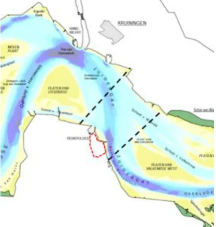
(8) 1.2.Case description The Perkpolder is located in the middle of the Western Scheldt (Figure 1.1). In 2003, the Kruiningen-Perkpolder ferry service was abandoned, because of the opening of the Westerschelde tunnel,. The previously busy Perkpolder port became deserted. The Perkpolder project plans to bring new life to the area by creating a recreation area including a luxury hotel, holiday residential units and golf courses (Figure 1.1). Moreover, the old dike was breached to create a new intertidal area. It aims at compensating for the nature loss due to the deepening of the Western Scheldt and adding ecological value by creating estuarine nature.. Figure 1.1 Map of Scheldt estuary (van der Werf & Briere, 2013) and the schematization of the Perkpolder plan. The dash line indicates the extent of the Perkpolder intertidal area.. Firstly, new dikes were built in 2014 around the previous agriculture area. Secondly, the creeks were shaped in the same year before breaching the dikes to make sure the immediate response of natural evolution after the flow entered the area. The design plan for the creeks is the results of the workshop in the cooperation of Rijkswaterstaat (RWS), province Zeeland and water board Zeeuws-Vlaanderen (Delta Expertise, 2013). Near the breach inlet, a pond was dug to -3 m NAP (Figure 1.2). This pond was considered as part of the creeks. Further inland, more creeks were created. According to the bottom width and depth of the creek, these creeks can be categorized into three types (Figure 1.2 The overview of creek system in the Perkpolder intertidal area). The first types are the major inland creeks which connected to the pond. The second types are the branches of the major inland creeks and the third ones are the terminals of the creeks. The detailed information of width and depth of the different creeks can be found in Table 1.1. Table 1.1 Design value for different types of creeks TYPE 1 2 3. DEPTH -1.50 m NAP -1.23 m NAP -1.00 m NAP. 8. BOTTOM WIDTH 10.0 m 5.0 m 2.5 m.

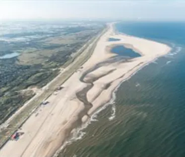
(9) Figure 1.2 The overview of creek system in the Perkpolder intertidal area (Delta Expertise, 2013).. In the early 2015, a unique seepage facility was installed to protect freshwater in the surrounding agricultural area (De Louw, 2015). After that, the breaching of the old dike was executed. Firstly, the crown of the old dike was removed. The dike was excavated to a lower level over the length of 400m. Moreover, a small channel was created in the middle of the breach which allowed tides to enter the area on the 25th of June, 2015 (Figure 1.3).. Figure 1.3 The first inflow through the breach. Besides the execution of the project, a monitoring plan was also issued. The monitoring plan (from 2015 to 2018) covered the geomorphology, hydraulic, groundwater, benthos, birds, vegetation and soil (Centre of Expertise Delta Technology, 2015). The data provides necessary information for completing the Master’s Thesis Project which is part of the Centre of Expertise Delta technology-project.. 9.

(10) 1.3.Research objective and questions The objective of this MSc project is: To document and understand the morphological development by investigating the influence of breach width and artificial creeks on morphodynamics in the Perkpolder intertidal area, the first nine months after being exposed to tidal influence.. Because the Perkpolder intertidal area is still in the early morphological stage, vegetation has not been well developed. Therefore, vegetation effect is outside the scope of this research project. Based on the research objective, the following questions are defined: 1. What are the relevant aspects regarding drivers, concept of and obstacles to managed realignment? 2. what are the hydrodynamics (tidal prism, flow fields) and morphodynamics (inlet development, bed level changes and sediment volume changes) based on the measured data? 3. How well can the Delft3D model reproduce measured hydrodynamics and bed level changes in the Perkpolder intertidal area? 4. What are the main processes which govern the sedimentation and erosion pattern and how could artificial creeks and breach width and artificial creeks influence the morphodynamics?. 1.4.Research approach Firstly, a literature review was conducted to gain background information into managed realignment project which answers the first research question in Chapter 2. After that, the monitoring data of the Perkpolder intertidal area are introduced and analyzed in Chapter 3. The analysis provides the input for the model setup and acknowledge of the morphological development in the fields. Therefore, a numerical delft3d model was built which simulates the hydrodynamics and morphodynamics. The model setup is introduced in Chapter 4. It is a depth-averaged concept model which considers tides as the major driven force and includes sand-mud interaction. The model was calibrated to show its ability of reproducing the measured velocity at the inlet and the observed sedimentation and erosion pattern. The model performance is assessed in Chapter 5. Chapter 4 and Chapter 5 in cope with the forth research question. As the model proved its skill, the model was used to understand the morphological changes in the Perkpolder in Chapter 6. Moreover, the different design choices of artificial creeks and breach width are simulated to show their influence in morphological development in the Perkpolder intertidal area in the same Chapter. In the end, besides the discussion, conclusion and recommendation were given in Chapter 7, 8 and 9 representatively.. 10.

(11) 2.. Chapter 2 2. Managed realignment 2.1.Drivers Recent years, sea level rise, climate change and human intervention have posed a challenge to water management regards sustainability and safety. The traditional ‘hold the line’ policy in coastal area is no longer recognized as a long term sustainable strategy. Most of the Dutch coast is protected by sand dune and the hard structures like sea walls and barriers are considered for the rest of the coastal area in the Netherlands (Mulder, et al., 2011). Due to the sea level rise and climate change, the coastline is migrating landward and the erosion from the Dutch coastline and the dikes has increased. The approach of focusing on increasing the strength by adding armor and rising the height of the defences has disadvantages. The high cost of maintaining and upgrading of the defences is not economically viable. Moreover, the coastal squeeze has placed an increasing threat on the Dutch coastline. The coastal squeeze is the process which the coastal margin is squeezed due to the sea level rise and fixed landward boundary by defences. It constrained the resilience of coastline. As a consequence of all the problems, the coastal environment and biodiversity have been degraded (Valiela & Fox, 2008). In the rivers and estuaries, the challenge lies in dealing with the higher water level and larger discharge. It increases the risks of the failure for the existing defences (Mcgranahan, et al., 2007; Nicholls, 2004). Moreover, the ecological function and value in the river and estuary has been well realized. The traditional engineering approach of flood protection sacrificed natural habitats and led to undesired environmental impacts. For example, the Western Scheldt, in the Netherlands and Belgium, is one of the estuaries which is subject to environmental deterioration due to human intervention such as land reclamation, reinforcement of dikes and maintenance of navigation channel by dredging and disposal (Wang, 2015). Compare to the situation in 1900, about 2500 ha of estuary natures (mudflats and salt marshes) in the Western Scheldt have been lost (Eertman, et al., 2002). The concern for conservation of natural habitats and the maintenance of biodiversity has led to the adoption of the Birds Directives (The European Parliament and the Council of the European Union, 2009) and Habitats Directives (The Council the European Union, 1992). The directives aim at no loss of species and protected intertidal habitats. The publication of the EU nature legislation allocates the responsibility to the member states in the European Union. Therefore, for the foreseeable future, a new strategy which is robust in environmental, social and ecologic is urged to be issued. Managed realignment is raised as an alternative plan to the traditional approach.. 2.2.Concept 2.1.1 Definition Although the oldest managed realignment schemes in Europe were implemented in the 1980s, there are only a few systematic studies of the concept. The inconsistent use of the terminology can be found in the literature. The book of “managed realignment: A Viable Long-Term Coastal Management Strategy?” (Esteves, 2014) is the first book which provides the overview of the managed realignment concept and projects. The book indicated that the 11.

(12) understanding of the term has evolved was evolving through time and the universal definition of the term is still missing. However, Esteves (2014) proposed a new possible definition as: “Managed realignment is a soft engineering approach aiming to promote (socio-economic, environmental and legal) sustainability of coastal erosion and flood risk management by creating opportunities for the realisation of the wider benefits provided by the natural adaptive capacity of coastlines that are allowed to respond more dynamically to environmental change.”(p.28) The phrase is commonly used in UK, while in the other countries, it appears as different names, like ‘set back’, ‘managed retreat’, ’de-embankment’ or ‘depoldering’ (French, 2006).. 2.1.2 Categories Managed realignment projects can be categorized into three major groups as removal of defences, breach of defences and realignment of defences (Esteves, 2014). Each category will be explained below with one example project. Removal of defences is implemented as the entire sections of the defences are removed, along with the new defences which are built landwards. By removing the old defences, the area can be flooded and can develop into nature area. Such implementation can be found on the South Devon coast, in south of Brixham, UK. The project is called ‘Man Sands’ which was completed in 2004. The deteriorated defences were removed (Figure 2.1). The absence of the old defences allowed tides enter the previously protected land which created about 2 hectares of wetland (Esteves, 2014). This additional habitat areas attracted birds (e.g. swallows) and local birdwatchers (Figure 2.2).. Figure 2.1 Managed realignment site 'Man Sands' after executed, UK (Anon., N.D.).. Figure 2.2 Local birdwatchers visit the bird hide at Man Sands (Anon., N.D.). Breach of defences is implemented as the selected sections of the existing defences are removed. It is similar to the category of removal of defences, the difference is the remaining amount of the previous defences after realignment. The breaching of defences can happen naturally or artificially. The Netherlands is one of the first three countries conducted managed realignment projects in Europe. In 1990, the summer dike in the Sieperda polder of the Scheldt estuary, the Netherlands, was breached by severe storms. The decision was made that the dike would not be repaired and the area was exposed to tides (Eertman, et al., 2002). Afterwards, vegetation colonized the area quickly (Figure 2.3).. 12.

(13) Figure 2.3 vegetation colonization of managed realignment project ‘Sieperda polder’, the Netherlands (Eertman, et al., 2002).. Realignment defences is determined when the line of defence changed position landwards. This realignment project is usually considered as the current defences cannot in cope with the sea level rise. Instead of updating the defences, new defences are built further inland while the current defences are abandoned. Overflow will happen naturally with time, thus the area behind the defences will be inundated. Moreover, the method of adding buffer in front of the defences is also considered as part of this category. Although in this case the defence won’t be moved, by creating new ‘land’ in front of the defence, the relative position of the defence is changed. One of the typical examples is the Sand Engine (also known as ‘Sand Motor’) project in the Netherlands. Sand Engine project belongs to the Building with Nature program. During the project, 21.5 million cubic meters of sand was placed in front of the coast of Zuid-Holland between Hoek van Holland and Scheveningen in 2011. This artificial sand bank is called the Sand Motor (Figure 2.4). It functions as a buffer for storm impact and leads to the creation of natural and recreational area (Vikolainen, 2012; Anon., 2014).. Figure 2.4 ‘Sand Motor’ in 2015, the Netherlands (Anon., 2014). 13.

(14) 2.3.Obstacles 2.3.1. Risks and Uncertainties Managed realignment is implemented in various countries like United Kingdom, the Netherlands, Germany and United State of America. Due to the different local boundaries and initiatives, the methods, sizes and design concepts vary among the projects. The small projects are only a few hectares like the Paddebeek Project in Belgium of 1.6 ha. While the Anklamer Stadtbruch project in Germany focused on 1750 ha nature area (Esteves, 2014). The variables in the managed realignment projects increase the risks and uncertainties. The success of the managed realignment cannot be assessed right after the completion of the implementation. Thus the monitoring and maintaining cost could claim a large amount of the budget. Until now, for most countries, managed realignment is still a “learning by doing” strategy. The restoration of flora is the common goal of the managed realignment project. However, vegetation colonization is a relative slow process. Angus and Mineke (2008) surveyed fourteen abandoned reclamations and four managed realignment sites along the Essex coast, UK. Over a century, the plant communities showed 10.5% similarity to the reference marsh communities. Vegetation cover has the function of attenuating the waves and acting like a buffer in front of the secondary defences. However, vegetation requires time and maintenance to reach a sufficient density for protection. The design choices in the managed realignment project lack of guidance. Natural processes need to be translated into the design principles. The resilience of the area can be obtained by the smart design. However, as an innovation approach, no lessons have been learned from other projects. Thus the impact of the design choices lead to large uncertainties which hesitates the decision makers.. 2.3.2. Stakeholders Managed realignment needs support from stakeholders. It usually evolves multiple stakeholders. The communication between the stakeholders is challenging. Managed realignment is not a generic plan which has its limitations. NIMBY (’not in my backyard’) attitude is commonly seen among the stakeholders and some stakeholders even against it. In 2011, the European Commission expressed their concern of nature conservation due to the on-going deterioration of habitats in the Natura 2000 site ‘Westerschelde & Saeftinghe’ in Western Scheldt. Thus the European Commission sent a letter to the Dutch government about the urgent ecological requirements of nature restoration in the Western Scheldt. In response, the Dutch government proposed a development plan for several managed realignment projects which contribute about 600 hectares of estuarine nature in Western Scheldt (The Netherlands. Minister for Agriculture and Foreign Trade., 2012). The plan included the Hedwigepolder project. However, due to the resistance from the stakeholders, the project was delayednever starts. In 2016, the Council of State made the final decision that the Hedwigepolder must be inundated in 2019. the policy on nature compensation should pay more attention to eliminate the resistance and ensure the successful engagement of the stakeholders.. 14.

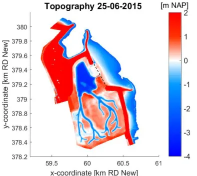
(15) 3.. Chapter 3 3. Data analysis Firstly the monitoring data is presented. Afterwards, the methodology which was used in this preojct is introduced. In the end, the result are shown in this Chapter.. 3.1. Field data 3.1.1. Multi-beam and laser data. The intertidal area and the inlet surroundings were measured by Rijkswaterstaat (RWS) as part of the monitoring program. The first available bathymetric data (T0) is a combination of measurements by the contractor and RWS. The inlet surroundings have been measured by RWS utilizing multibeam sonar in May 2015. The new intertidal area has been measured by the contractor directly after breach. As no clear inlet channel has formed in the inlet surroundings, the inlet surroundings must have been measured close to the breach date. Therefore, the T0 data set can represent for the situation when the dike was removed. However, the T0 topography has some inconsistencies. Figure 3.1 shows that the old dike in the North of the inlet channel has been lowered more than the Southern part, however figure Figure 3.2 shows that both sides of the inlet were similar at the time of breach.. Figure 3.2 The situation of the breach on 25-06-2015. Figure 3.1 Overview of topography at T0, the dash line indicates the discrimination of two data sets measured at different time.. Afterwards, the morphological development of the study site was monitored several times by RWS (Table 3.1). However only part of the Northern part of the inertial area and inlet surroundings were measured (Figure 3.3). The different resolution between T0 and the other 15.

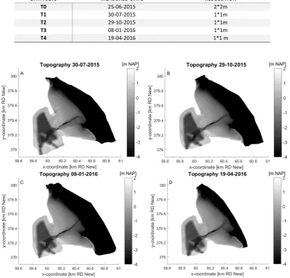
(16) measurements is due to the interpolation by RWS of the multi-beam measurements. The data was recorded by multi-beam and the extent of the monitored area varied over time. The measurement data has been collected utilizing the Dutch national triangulation system as coordinate system. Table 3.1 Overview of the monitoring data DATA SETS T0 T1 T2 T3 T4. MEASURED DATE 25-06-2015 30-07-2015 29-10-2015 08-01-2016 19-04-2016. RESOLUTION 2*2m 1*1m 1*1m 1*1m 1*1 m. Figure 3.3 Overview of the topography of the Perkpolder intertidal area over time. (A) Topography with data sets T1 (30/07/2015). (B) Topography with data sets T2 (29/10/2015). (C) Topography with data sets T3 (08/01/2016). (D) Topography with data sets T4 (19/04/2016).. 3.1.2. Point measurements 3.1.2.1. Inlet A seven-day data series of the currents through the inlet is available, which has been measured with pressure sensors by RWS. The sensors measured the depth-dependent horizontal flow velocities and water level every ten minutes from 2015-11-25 12:00 to 2015-12-01 14:30. The velocities were calculated in depth average and the directions of the velocities were determined as the full cycle (0° to 360°, clockwise) with 0° heads to the North by RWS. The six measurement locations were placed along the inlet (Figure 3.4). Moreover, the cross-section of the inlet was also measured by students from HZ University of Applied Sciences on 25-11-2015 using Differential Global Positioning System (DGPS) (Figure 3.). The measurement started at one of the remaining dike and ended with the other one. The 153. 16.

(17) DGPS measurement points were located more concentrated to the Northern part while the inlet channel was not measured due to the safety issue as the channel is too deep.. Figure 3.4 The locations of the measurements at the inlet with the topography of T0. The markers indicates the pressure sensor locations and the black points are the locations measured by DGPS.. 3.1.2.2. Intertidal area The sedimentation inside the intertidal area was measured by Martens (2016) on 28-04-2016. The method is based on the assumption that the initial bed layer inside the Perkpolder is non-erodible, compacted peat. A bamboo stick which has the radius of 2cm is pushed into the soil. The height of the stick penetrated the soil until it reached the solid surface is considered to be the sedimentation thickness. The sedimentation thickness was recorded at 545 locations and the value at each location was determined by the average of five measurements.. 3.2. Methodology 3.2.1. Hydrodynamics 3.2.1.1. Tidal prism The tidal prism is determined by the high water slack and low water slack filling or emptying the basin which based on the theory that the current started to reverse about one hour after the high tide and low tide (Van Veen, et al., 2005). It can be calculated as: (1) Where P is the tidal prism (m3); LWS is the time of low water slack (s); HWS is the time of high water slack (s); Q is the discharge (m3/s); The discharge though the inlet is determined by the depth-averaged velocity which is perpendicular to the inlet and the cross-sectional area. The perpendicular angle for the outflow is assumed to be 60°. As shown in Figure 3.4, the velocity measurements are approximately in line with the DGPS measurement locations and the cross-section area determined by the DGPS was measured on the start day of the velocity measurement period. Therefore, the discharge can be. 17.

(18) calculated as: (2) 3. Where Q is the discharge (m /s); is the perpendicular velocity at the velocity measurement MP010i; (m2) is the cross-sectional area determined by the measured water level and the bed level which was measured by DGPS (Figure 3.5);. Figure 3.5 Determination of the cross-sectional area. 3.2.1.2. Flow fields The flow fields include the magnitude and direction of the velocities at the six measurement stations. The velocity vector as arrows are determined by u components (perpendicular to inlet) and v components (parallel to inlet) with a scale factor of 0.2 in Matlab. It is assumed that the flow direction 60° from North is the flow leaves the inlet perpendicularly (positive u component).. 3.2.2. Morphodynamics 3.2.2.1. Inlet development As the DPGS measurement clearly indicates the location of the remaining dikes, it regards as a reference. Thus a calculation line for the cross-section at the inlet is determined by the two ends of the DPGS locations. 1000 points along the line which have equal distance of 0.43m are used to determine the cross-section area at different time. Moreover, the cross-sectional area of the inlet is compared with the empirical equilibrium area. The determination of the equilibrium area is calculated based on the equation by Hughes (2002) as: (3) Where is the minimum equilibrium cross-sectional area (determined as the area below mean sea level, m2); is the tidal prism corresponding to the diurnal or spring rang of tide (m3) and the highest tidal prism derived from the current measurement is represent for the spring rang of the tide in this report.. 18.

(19) 3.2.2.2. Bed level changes The bed level is measured utilizing difference data sources, therefore different approaches are used to analyze the bed level change. Firstly, the focus is on the morphological development after the dike was breached, this is done for periods between measurements of the intertidal areas. In the area which is more frequently measured, the bed level changes are determined by the difference in topography data sets at each cell using ArcGIS. The output raster has a resolution of 1m. The positive values represent sedimentation and negative values represent erosion. While for the area measured by the bamboo stick, only sedimentation was measured. The results are plotted on top of the initial topography to show the sedimentation pattern spatially. Besides the overview of the bed level changes since the dike was breached, the changes of the sedimentation and erosion rate over time are calculated. The rate (m/day) is determined as the bed level changes over the measurement periods (Table 3.1). In this case, only the multi-beam and laser data is considered as it was measured five times. Table 3.1 The overview of measurement periods. Index 1 2 3 4. Measurement period 25/06/2015-30/07/2015 30/07/2015-29/10/2015 29/10/2015-08/01/2016 08/01/2016-19/04/2016. 3.2.2.3. Sediment volume analysis The sediment volume analysis is used to understand the volume changes inside and outside the Perkpolder intertidal area and determine the sediment flux through the inlet. As the intertidal part was measured differently, the volume analysis is focus on three parts (Figure 3.6). Part1 represents for the outside area while intertidal area consists of part2 and part3. As part3 was only measured by points, the points measurement has to be interpolated to the extent of part3. . The Inverse Distance Weighted (IDW) interpolation method in ArcGIS which determines the value based on the line-weighted combination is considered. Each cell is determined by the surrounding 12 points and the further away the less influence of the point.. Figure 3.6 Overview of the three parts. 19.

(20) The volume changes (m3/m2/day) for part1 and part2 are determined as the cumulative sediment volume change per area during each measurement period (XX). As the measurement period for part3 is from 25-06-2015 to 28-04-2016 which not only includes the four multi-beam and laser measurement periods (25-06-2015 to 19-04-2016) but also has 9 extra days. The volume changes for part3 at each multi-beam measurement period need to be determined. The assumption was made that the bed level change for the extra 9 days is negligible and the cumulative volume change for part3 is proportional to the part2 at each measurement period. The relationship can be determined by the equation (4): (4) Where is the cumulative sediment volume for measurement period i at part3; cumulative sediment volume for measurement period i at part2. is the. 3.3. Results 3.3.1. Tidal prism Discharge through the inlet and the tidal prism is shown in Figure 3.7 and Figure 3.8 respectively. The negative values of the discharge represent for flow into the perkpolder. Due to the asymmetric behavior of the discharge, the Perkpolder intertidal area is flood dominant. As for the tidal prism, it varies from 1.3 million m3 to 2.2 million m3. Tidal prism is influenced by the water level, bathymetry and perpendicular velocity through the inlet. The average tidal prism is 1.67 million m3.. Figure 3.7 Discharge through the inlet. Figure 3.8 Tidal prism over time. 3.3.2. Flow fields The flow fields (Figure 3.9 – Figure 3.14) indicates that bathymetry has large influence during ebb for low water level. The tidal start with an inflow through the major inlet channel and followed by the inflow through the secondary inlet channel which is located at the Northern part of the inlet. After the water level exceeds the bed level, flow enters the area through the entire inlet. However the velocity direction at each measurement location varies. Only the Southern two stations (MP1015 and MP0106) have the same velocity orientation, while the flow directions at rest stations are towards the extension of the major inlet channel. This discrepancy in velocity also can be seen during outflow. During outflow, instead of the Southern two stations, the Northern four stations have the same velocity direction. It can be expected the boundary influence the flow fields. Moreover, similar like flow enters the area, the two inlet channels lead the way of outflow 20.

(21) propagation.. Figure 3.9 The inflow in the major inlet channel. Figure 3.10 The appearance of the inflow in the secondary inlet channel. Figure 3.11 The flow fields during the high water. Figure 3.12 The flow fields during the outflow. Figure 3.13 The outflow during low water. Figure 3.14 The similar outflow pattern as inflow. 21.

(22) 3.3.3. Inlet development. Figure 3.15 The inlet development over time. The results (Figure 3.15) of the inlet development show that the major inlet channel is located between velocity measurement location MP0103 and MP0104. Since the breach the major inlet channel became wider and deeper. Furthermore a secondary channel formed between MP0101 and MP0102 after the dike was breached. The evolution of the breach inlet shows a clear difference in the location of the dike, which can be observed clearly in the DGPS measurement and T0 measurement. This indicates the dike at the northern and southern end of the cross-section is measured incorrect at T0, as the dike are armoured structures which cannot be eroded. Moreover, the cross-sectional area which is below the mean sea level is compared with the empirical equilibrium value from equation (4). The area increased dramatically in the first measurement period, afterwards the breach inlet started to stabilized. It is almost stable for the last two month of 2015 and slight increased again in 2016. The cross-sectional area is however significantly lower than the equilibrium area of around 170 m2.. Figure 3.16 The comparison of the minimum cross-sectional area with the equilibrium value. 22.

(23) 3.3.4. Bed level changes 3.3.4.1. Pattern. Figure 3.17 The overview of the morphological development.. There is a small elevated area in the pond which is noticeable at topography of 25-06-2015. It was the results of the artificial soil redistribution inside the area. The pond and this elevated area is indicated with the contour line (-2m NAP at T0, dashed line in Figure 3.17). It can be observed clearly that the pond which initially had the lowest elevation accretes quickly. However, the sedimentation inside the pond does not spread out evenly. A channel with around 0 sedimentation can be visualized. This could be the results of the high velocity which can be observed at the flow fields (Figure 3.10). Erosion took place on the edge of the elevated area inside the channel, due to the high velocities in the channel. The major inlet channel outside the perkpolder was also eroded and the channel changed the orientation outside from Southeast to Northeast. As for the sedimentation inside the Perkpolder intertidal area, in general, the Eastern part of the area has higher sedimentation than the Western area (Figure 3.18). However, the high sedimentation was constrained along the creeks, especially the rear of the area. Only around 10 cm sedimentation was found in the creek banks. In the Southwest corner, around 25cm sedimentation spread out more evenly.. 23.

(24) Figure 3.18 Sedimentation further inland measured by bamboo stick. 3.3.4.2. Rate. Figure 3.19 Sedimentation rate at different measurement period. 24.

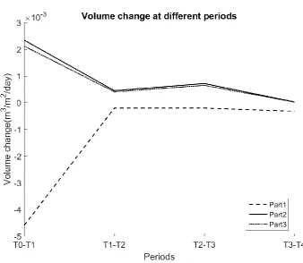
(25) In general, morphodynamics were highly active at the beginning (Figure 3.19). The biggest changes were observed from T0 to T1 (Figure 3.19 A) after the dike was breached. The sedimentation rate inside the pond dropped from 2 cm/day to around 2 mm/day. While for development of the major inlet channel, only the slight widening can be observed after July,2015. 3.3.4.3. Sediment volume analysis. Figure 3.20 Volume change at different measurement period. Table 3.2 Overview of the volume change. Volume changes (m3/m2/day). 25-06-2015 to 30-07-2016. 30-07-2015 to 29-10-2015. 29-10-2015 to 08-01-2016. 08-01-2016 to 19-04-2016. Part1 Part2. -4.60e-03 2.34e-03. -2.05e-04 4.48e-04. -2.04e-04 7.17e-04. -3.24e-04 2.56e-05. 2.12e-03. 4.06e-04. 6.49e-04. 2.17e-05. 5.00e+04. 2.94e+04. 3.11e+04. 1.45e+03. Part3 3. Flux (m ) Part2+Part3. As expected from the sedimentation and erosion rate, the largest volume changes for all the parts are found from 25-06-2015 to 30-07-2015 ( Figure 3.20 and Table 3.2). It is one or two magnitude higher than the changes for the rest of the periods. It could due to the influence of sediment redistribution after the dike was breached and the inlet channel is formed. More erosion than sedimentation happens outside the Perkpolder area (Part1). The volume change for outside the area is stable after July in 2015. However, the volume change inside the Perkpolder area (Part2 and Part3) is different in these months with larger values in winter. It indicates that the sediment supply is higher in winter for the Perkpolder intertidal area. 25.

(26) For the first 4 months in 2016, more erosion took place in the outside area. However, at that period, the smallest positive volume change can be observed for inside area. This could be due to the influence of the storm. The non-linear relationship of the flux through the inlet between the periods is not as obvious as the volume changes. However, the smallest flux is also found in the last measurement period. The flux is important for the model calibration which will be further discussed in Chapter 4.. 26.

(27) 4.. Chapter 4 4. Model setup 4.1. General The Western Scheldt is a tide-dominated estuary as the tidal prism is about 500 times larger than the discharge of river Scheldt (De Vriend, et al., 2011). The Perkpolder intertidal area is in the more sheltered part of the Western Scheldt. The area is protected by groynes, therefore it is believed that the wind and wave have minor impact on the area, while the tides are the major driving force. Moreover, both sand and mud transport are active near the Perkpolder (Dam & Cleveringa, 2013), the sand and mud interaction should be taken into account. Moreover, as the deposition of the sediment from the Scheldt is more important for the long-term morphological development than the initial sediment redistribution, the Perkpolder model is considered to be a depth-averaged model which aims at simulating the morphological development due to sediment supply. The Perkpolder model is implemented in the process-based Delft3D-FLOW module. The Delft3D-FLOW model requires hydrodynamic and sediment boundary conditions, these boundaries can be provided by a regional model. This method, called nesting in Delft3D-FLOW, was used in this project to obtain time-series and more accurate hydrodynamic boundary conditions for the detailed Perkpolder model. The Delft3D-NeVla model was used to generate the hydrodynamic boundary conditions, which will be introduced later. The sediment boundary conditions were determined differently. The Perkpolder model simulates the sand-mud interaction which requires separate boundary conditions for each sediment type.. 4.2. Delft3D-NeVla model The NeVla model is a detailed depth-averaged (2DH) flow model which covers the Scheldt estuary. The model is developed from the NeVla-SIMONA model and incorporated into Delft3D by Grasmeijer (2013). The NeVla model used in this project has been calibrated by Vroom et al. (2015) and further developed by Vroom (2016) to simulate the situation in 2014. The hydrodynamics is calculated by the model on the basis of the tide in the North Sea, currents of the upstream rivers and wind. One representative spring and neap cycle with a duration of 14 days 23 hours and 40 minutes was used in NeVla model based on the ratio between the amplitudes of spring and neap tide to represent for the year 2014. As the NeVla model is used to generate the hydrodynamics boundary condition for the Perkpolder model. The NeVla model was re-run with a rough schematization of the Perkpolder intertidal area to minimize the influence of the Perkpolder intertidal area on hydrodynamics.. 4.3. Perkpolder model 4.3.1. Domain The choice of the study domain is based on the consideration of the computation time, the requirement of excluding the intertidal part at the boundaries and the flow should enter the boundary perpendicularly. The detailed Perkpolder model consists of the Perkpolder intertidal. 27.

(28) area and the surroundings including the channels in the Western Scheldt estuary (Figure 4.1).. Figure 4.1 The overview of Perkpolder surroundings. The red dash line shows the location of the Perkpolder intertidal area and in between of the two black dash lines, including Perkpolder intertidal area, indicates the domain of the Perkpolder model.. 4.3.2. Grid The Perkpolder intertidal area was extended from the outside area as determined by Nevla model. Firstly, the outside part was derived from the whole extent of the Nevla model. After a coarse schematization of the Perkpolder intertidal area, the whole grid was refined to a resolution of 3 by 3 meters to cover the small creeks inside the area. Moreover, the whole grid was orthogonalised to fulfill the requirement of orthogonality in the Delft3D-FLOW module. The resolution is defined as the square root of grid cell area (m) in Delft3d-RGFGRID manual (Deltares, 2014). As the rectangle grid is not complete square, the resolution is just the indication about the size of the grid. Due to the method used in this project to build the grids, the differences between the girds outside and inside the Perkpolder intertidal area are relatively small. The general grid outside is about 20m by 20m and the grid inside the Perkpolder intertidal area has the general resolution of 18 by 18m. The resolution is sufficient to schematization the creeks inside which is further discussed in the Bathymetry section. 4.3.3. Bathymetry The bathymetry data of the surroundings of the Perkpolder intertidal area is obtained from the Nevla model, which is based on the measurement of 2013. The bathymetry data of Perkpolder intertidal area is the measured topography which was exported from ArcGIS. As learned from the Chapter4, the T0 has minor inconsistencies, which influence the morphological development of the Perkpolder. The focus of the Perkmodel is to replicate the long term effects of the managed realignment project, therefore it has been chosen to utilize T1 as the initial bathymetry. In Figure 4.2 of the Perkpolder intertidal area, the creeks and the major inlet channel can be clearly observed.. 28.

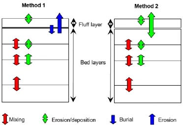
(29) Figure 4.2 The overview of the Bathymetry. 4.3.4. Groynes The groynes are placed outside the Perkpolder intertidal which influence the sediment transport. Although the bathymetry indeed shows the location of the groynes with high bed levels, however the erosion could happen at the location. As the groynes are non-erodible, the thin dams are used to schematize the groynes. 4.3.5. Hydrodynamics Tides are the major driving force for the Perkpolder model. The tides are simulated by imposing corresponding hydromantic boundary conditions. The flow is forced using water level (downstream) and current (upstream). Consideration the spatial difference along the open boundary, the downstream boundary was divided into 10 sections while the upstream was divided into 9 sections. The boundaries were obtained by nesting tools in the Delft3D-FLOW module. Each end of one boundary section is determined by four surrounding monitoring stations in the Nevla model with different weights. It results in one representative spring-neap cycle for the Perkpolder model. This spring-neap cycle is repeated for the whole simulation period. The nesting method will be further discussed in Chapter 5 with the model results.. 4.3.6. Morphodynamics 4.3.5.1. Bed stratigraphy A single, well mixed bed layer is chosen for Perkpolder model. Besides the bed layer, a so called fluff layer was used to replicate the dynamics of the cohesive sediment (mud) during the slack water (Van Kessel, et al., 2012). Within the low-high tide cycle, the fluff layer is able to capture the rapid sediment exchange between the fluff layer and the water column while the bed layer changes slowly. The fluff layer only influence the cohesive sediment and it does not contribute to the bed level. There are two types of fluff layer, the difference between the types is the exchange between the fluff layer and bed layer (Figure 4.3). In the first type of fluff layer, the deposition comes from the fluff layer, which was determined by a burial term. The second type directly deposits sediment from the water column to the fluff layer. In both types, sediment can be eroded from fluff layer and bed layer. The eroded sediment becomes suspended in the water column. Due to the different concept, the sedimentation equations for the fluff layer and bed layer are different 29.

(30) with the fluff layer type. While the erosion equations are the same (detailed explanations see (Van Kessel, et al., 2012)). In this project, method 1 gives more control of sedimentation from fluff layer to the bed using burial coefficient. This type was chosen to achieve the similar spatial patterns in sedimentation of Perkpolder intertidal area and the estuary outside the area (see Chapter 5).. Figure 4.3 The concept of two types of fluff layer (Van Kessel, et al., 2012).. 4.3.5.2. Boundary The Perkpolder model has multiple sediment fractions, thus sediment supply of cohesive sediment (sand) and non-cohesive sediment (mud) is required at the boundaries. The sand concentration at the boundaries is set to the equilibrium concentration, While the mud transport data is obtained from the mud model which is developed by Van Kessel et al (2008). The mud model simulated the mud transport in 2006 (from 5th of Jan, 2006 to 1st of Jan, 2007) which focused on the sediment concentration patterns. The seasonal dynamics of the mud content was well reproduced by the model with low mud contents in winter and higher mud content in summer. However, the model underestimated the cross-sectional uniform fine sediment concentrations. The modelled concentration at low water has a range of 100 to 160 mg/l at boei84 which is near Antwerp at the upstream of the Western Scheldt. While the monitoring data shows the concentration from 100 to 1000 mg/l (Van Kessel, et al., 2008). This underestimation of mud concentration gives an indication that the sediment supply derived from the mud model might be too low for replicating the morphological development in the fields. The computed total inorganic matter at locations Hansweert and Baalhoek are used to determine the downstream and upstream boundaries respectively. The computed values are subjected to the calibration, which will be further discussed in Chapter 5. 4.3.5.3. Sediment transport The cohesive sediment can only be transported as suspended load. While both suspended load transport and bed load transport can be found for the non-cohesive sediment. The suspended load transport is determined by solving the three-dimensional advection and diffusion. 30.

(31) equation (5).. (5) Where is mass concentration of sediment fraction (kg/m3); is flow velocity components (m/s); is eddy diffusivities of sediment fraction (m2/s); is (hindered) settling velocity of sediment fraction (m/s), determined as with. is the reference density (kg/m3),. settling velocity for sediment fraction the sediment fractions.. (m/s),. is the ‘basic’ specific. is the sum of the mass concentration of. The transport formulations of Van Rijn et al. (1993) were chosen for non-cohesive sediment. The method regards the transport below the calculated Van Rijn’s reference height as the bed-load transport, otherwise it is referred to as the suspended transport (Deltares, 2014). 4.3.5.4. Sediment erosion and deposition For cohesive sediment, the erosion and deposition is influenced by the fluff layer. The deposition in the water column to the fluff layer is calculated by equation (6) and the deposition from the fluff layer to the bed is calculated by equation (7).. Where is deposition flux of mud fraction efficiency (-); is settling velocity (m/s) and 3 column (kg/m );. (6) to fluff layer (kg/m2/s); is deposition is concentration of mud fraction in water. (7) Where is burial flux for mud fraction from the fluff layer to the first bed layer (kg/m2/s); is mass fraction of mud fraction in the fluff layer (-); is total mass of the fluff layer per unit area (kg/m2); is burial coefficient 1 (kg/m2/s); is burial coefficient 2 (s-1); The erosion from fluff layer and the bed layer to the water column is influenced by the erosion coefficient, critical bed shear stress and bed shear stress (see equation 8 and 9). However, different erosion coefficients are considered for different processes and the critical shear stress of the erosion from fluff layer has to be smaller than the bed layer as it has to be more dynamic. (8) Where is erosion flux of mud fraction from fluff layer (kg/m /s); is mass fraction of mud fraction in the fluff layer (-); is erosion parameter (s/m) which is determined as with as total mass of the fluff layer per unit area (kg/m2); as 2 erosion coefficient 1 (s/m); as burial coefficient 2 (ms/kg); is bed shear stress (N/m ); is critical bed shear stress (N/m2); 2. (9) Where fraction (N/m2);. 2. is erosion flux of mud fraction from bed layer (kg/m /s); is mass fraction of mud in the bed layer (-); is erosion coefficient (kg/m2/s); is bed shear stress 2 is critical bed shear stress (N/m );. For non-cohesive sediment, the erosion and deposition is simulated with sink and source terms, which is acts on the above reference height near-bottom layer. The sink term is solved 31.

(32) implicitly in the advection-diffusion equation each half time-step. The source term is solved explicitly during each time-step (Deltares, 2014). 4.3.5.5. Sand-mud interaction The sand-mud interaction is involved in Delft3D based on the user defined critical mud fraction. In Perkpolder model, the fraction is chosen as 0.3. Whenever the mud fraction is below the critical mud fraction, the regime is non-cohesive and the regime above this critical value is cohesive. The erosion flux was calculated differently in each regime. For non-cohesive regime, the erosion of flux is calculated based on the standard erosion formula and mud is proportionally eroded with sand. And for the cohesive regime, the sand is eroded proportionally with the mud and the mud flux is the interpolated results of flux in the non-cohesive regime and the fully mud situation (Van Kessel, et al., 2012).. 32.

(33) 5.. Chapter 5 5. Model assessment 5.1. Hydrodynamics calibration The hydrodynamics in the Perkpolder model were determined by the water level from downstream boundary and the currents of the upstream boundary. The boundary conditions are derived by the Nesting tools. The dry points should be avoided in the nesting method. The boundaries are divided to several segments.In each segment the boundary conditions are determined to maintain spatial differences. The calibration of hydrodynamics has been done by changing the number of the segments and their locations. The hydrodynamics in the Perkpolder model are determined by the NeVla model, which has the simulation period of 2014. It needs to be verified that how well the two models could reproduce the major tidal components for the measurement period of 29th of July, 2015 to 9th of January 2016 which is consist with the model simulation time. This verification was done with the tidal analysis tool by Pawlowicz et al. (2002). The tool converted the time-serial tide signal into different tide constituents (frequency, amplitude and phase) with 95% confidence. After the tidal component of the model is verified, the model is compared to the measured velocities and water levels near the perkpolder. At the six measurement locationsin the inlet the velocity is determined, these measurements have been introduced in Chapter 3.. Moreover, the modelled water level and velocity were compared with the observation points for outside the Perkpolder area. The best model results from the hydrodynamics calibration are shown in this chapter.. 5.1.1. Tidal analysis M2, S2, M4 and M6 are the major tidal components which determine the behavior of the hydrodynamics. As models and monitoring data are not in the same time period, the tidal phase is incomparable. However, regardless of individual phase difference, the relative phase of M2 and M4 ( ) which determines the tidal asymmetry is comparable. In the domain of the Perkpolder model, there is only one measurement station (Figure 5.1).. Walsoorden. Figure 5.1 Location of Walsoorden measurement station.. 33.

(34) Table 5.1 Comparison of tidal amplitude (m NAP) and relative phase (degrees) of M2, M4, S2 and M6.. NeVla model Perkpolder model Measurement. M2. M4. M6. S2. 1.97 1.98 1.99. 0.11 0.12 0.13. 0.08 0.08 0.10. 0.58 0.59 0.53. Relative phase -2.10 1.11 -7.15. The tidal analysis showed that the NeVla and Perkpolder model are quite comparable, only small small deviation can be observed in Table 5.1. The comparison of Perkpolder model and the measurement shows that the amplitudes of M4 and M6 tides are similar, however the model underestimates the amplitude of M2 tides for 1cm and overestimates the amplitude of S2 tides for 6cm. As the S2 and M2 tides are responsible for the formation of the spring and neap tides, the spring tides in the Perkpolder are slightly overestimated and the neap tides are slightly underestimated. The relative phase is higher in the two models than in the measurements. However, tidal analysis tool shows a large uncertainty in the calculated relateive phase (Figure 5.2). The uncertainty determined in this model is due to the non-tidal or residual noises from the signal. Due to this large error and the tidal analysis is only based on one measurement station, the model performance of both the Perkpolder model and the Nevla on hydrodynamics needs to be further determined.. Figure 5.2 The relative phase for the models and measurement with error bar. 5.1.2. Comparison of Perkpolder model and measurement Before the model results and velocity measurement in the inlet can be compared, a representative period needs to be determined. The monitoring station Walsoorden was monitored more regularly and the distance between the station and the inlet of Perkpolder intertidal area is relatively small, the representative period is determined by comparing the measured water level data and modeled results at Walsoorden. The criteria for choosing the best fit period is the Pearson coefficient (r) and RMSE (equation 10). RMSE describes the absolute deviation of the results with different weights to errors. The larger absolute error has larger weights than the smaller absolute error (Chai & Draxler, 2014). The higher RMSE value means the difference between two models are larger. The correlation coefficient r has a value range from -1 to 1. With an r value of -1, it means the two variables have negative correlation and the value of 1 means positive correlation. In other words, the higher r value, the more similar is the behavior of the two variables. No correlation is found if r=0, which indicates the variables is . The goal is to find the highest Pearson coefficient and smallest RMSE for the period of 7 days. (10). 34.

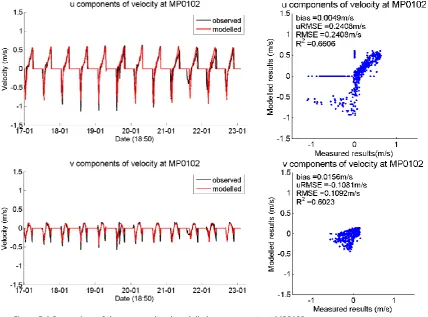
(35) (11) Where is the modelled results from Perkpolder model at time step ; is the modelled results from NeVla model at time step ; is the average value of the results from Perkpolder model; is the average value of the results from NeVla model; is the number of time steps; is the standard deviation of the results from the Perkpolder model; is the standard deviation of the results from the NeVla model. the best fitting period starts from 17-01-2014 18:40 to 23-01-2014 14:50 (Appendix), the modelled water levels and velocities at the corresponding location in the Perkpolder model were compared to the observed value. It is unknown whether the water level and velocity inside the Perkpolder intertidal area have delays compared to the best fit of Walsoorden. Therefore, the Pearson coefficient was calculated for various lag periods, ranging from +30 minutes to -30 minutes with an interval of 10 minutes. The results from the measurement station MP0102 are shown as an example (for the rest stations, see Appendix). The results indicate that a 10 minutes delay. Therefore, the final period for the comparison of Perkpolder model and monitoring data starts from 17-01-2014 18:50 to 23-01-2014 15:00.. Figure 5.3 comparison of water level and velocity at MP0102 with regards of time lag. In order to gain a more comprehensive overview of the velocity point comparison, perpendicular (u) and parallel to the breach (v) velocity components were compared separated. The determination of u,v of the measurements has been discussed in Chapter 3. The bathymetry data used in this model simulation was measured at 29th of October, 2015. The model was run as morphostatic, which prevents any morphological development in this period. The comparison for each measurement station has been assessed quantitatively with Bias, RMSE, uRMSE and R2 (equation 12-15). Bias indicates the average difference of results between two models. The positive bias means the Perkpolder model overestimates the velocity compared to the Nevla model and vice versa. RMSE describes the absolute deviation of the results with different weights to errors. The larger absolute error has larger weights than the smaller absolute error (Chai & Draxler, 2014). The higher RMSE value means the difference between two models are larger. The uRMSE is the bias corrected RMSE which is used when the distribution of error is unknown and also provide information of whether the results from Perkpolder model have a larger (uRMSE >0) or smaller standard deviation (uRMSE<0). The similarity in behavior of the two sets of water level is determined by R2. The R2 has the value between 0 and 1, with the value of 1, the data perfectly fits the regression line which created by the linear model. The higher R2 value means the closer linear relationship between the two data sets. 35.

(36) (12) (13). (14). (15) Where the variables have the same meanings as explained before. The measurement station MP0102 is used as example. It can be observed that there are a lot of zero points parallel to the x-axis and y-axis for the u velocity component (figure 5.4). When the model computes zero u velocity and the measured u velocity is negative, the inflow starts later in the model. When the zero value along the y-axis are observed when the outflow takes longer in the model than in the measurements. The difference in the bathymetry will lead to this result. As indicated in the water level comparison, the representation location in the Perkpolder model has higher bed level. The dynamics of the u-components are better reproduced than the v-components which is reflected by the higher R2 values. However, due to the smaller magnitude of the v value, it is harder to follow the observed value as a small deviation would result in smaller R2 value. Moreover, the morphological development was excluded for the hydrodynamics calibration. A larger difference could be observed for the 21st which could contribute to the large RMSE.. Figure 5.4 Comparison of the measured and modelled u,v compoents at MP0102. Besides the individual comparison at each measurement station, the accuracy of the 36.

(37) modeled velocity can be expressed by the Nash-Sutcliffe model accuracy (Nash & Sutcliffe, 1970). It is determined as: (16) NS score was calculated for the u,v components respectively at each measurement station (Figure 5.5). Horstman et al. (2015) categorized the model performance based on the NS score (Table 5.2). Table 5.2 The overview of model skill based on NS score.. MODEL SKILL. 0<NS<0.1 Poor. 0.1<NS<0.2 Reasonable/fair. 0.2<NS<0.5 good. 0.5<NS excellent. Figure 5.5 The NS score for all the u,v compoents. The results indicated that u components are excellently reproduced by the model while the v components have unstable performance. The v components for the measurement station MP0103 deviate from the others and has the lowest NS score here. In contrast, the model did an excellent job in reproducing the v-component at MP0102. In general, the model has good skill of replicating the measured velocities. Moreover, the NS score does not count for the relative difference. The u components are much larger value than the v components. The v components are responsible for the small deviation of perpendicular velocity direction towards the inlet. For simulating the morphological development, this deviation has relatively small influence on the sediment transport due to the numerical approaches in the model.. 5.1.3. Comparison of Perkpolder model and NeVla model The modelled water level and magnitude of velocity from Perkpolder model was compared with the results from NeVla model at six different measurement stations (Figure 5.6). The same four coefficients (Bias, RMSE, uRMSE and R2) are used to assess the model performance.. 37.

(38) Figure 5.6 Overview of the six observation locations. The summary information about the respective contribution of the bias and uRMSE regards to the RMSE is shown in the Taylor diagram (Jolliff, et al., 2009). It is based on the relationship between the three coefficients determined as: . The diagram has the x-axis of uRMSE and y-axis of bias while the RMSE is shown with different color (Figure 5.7 and Figure 5.8).. Figure 5.8 The Taylor diagram for velocity. Figure 5.7 The Taylor diagram for water level. The high uRMSE in the Taylor diagram implies that the Perkpolder has more variation in water level than the NeVla model. Due to the positive biases for all the locations, it can be concluded that the high water has larger difference for the two models. For the velocity, the three measurement stations in the deep channel have less variation than the other three stations. The Taylor diagram shows that the water level and velocity have high RMSE value at Walsoorden, which could be due to the influence of the Perkpolder intertidal area. While the largest deviation of velocity is found at MP DOWN, which could due to the influence of the water level boundary. However, beside the Walsoorden and the stations near the boundaries, the differences are limited.. 38.

(39) 5.2. Morphodynamics calibration Before conducting the sensitivity analysis, the model was run with the boundary derived from the mud model. This model has been introduced in Chapter4 and has been used to derive the boundary with both fluff layer type 1 and fluff layer type2. The modeled flux through the inlet is similar for both fluff layer type, the simulatd flux was close to 6.0 103 m3. This value is less than the interpolation results from Chapter3 as 3.89 104 m3. Since the model showed underestimation at the observation location, the boundary was initially increased with a factor of 3. However, with the triple mud boundary, the flux increased to 1.5e+04 m3. However, it is still less than half of the observed flux. It is unrealistic to get twice amount of the flux by changing parameters for fluff layer, the mud boundary was doubled again. The flux is further calibrated with the help of sensitivity analysis.. 5.2.1. Sensitivity analysis The sensitivity analysis is conducted with the focus on getting the correct magnitude of the flux through the inlet as calculated in Chapter3. Since the flux over time is almost linear, considering the computation time, the sensitivity runs have a simulation period of one month. The base run is considered without fluff layer as a simple case to gain understanding of the model (Table 5.3). Firstly, the basic parameters which influence the sedimentation and erosion process and the effect of the fluff layer are evaluated in the analysis. Since the fluff layer type 2 has no exchange of the fluff layer and bed, this layer is simpler and is used for the initial sensitivity analysis. Table 5.3 Overview of the parameters for first calibration round. Parameters. Base run. Settling velocity ( Erosion parameter for bed layer ( ) Critical shear stress for erosion for bed layer ( ) Reference density for hindered settling calculations ( ) Fluff layer (type 2). 0.001 m/s 0.0001 kg/m2/s 1 N/m2 1600 kg/m3. Range (value) at sensitivity run 25%, 50%, 200% 200%, 400% 50% 100 kg/m3. Without. With. The results showed that model is mostly sensitive for the implementation of the fluff layer. By including fluff layer, the flux increased about 50% (figure x). Moreover, decreasing the settling velocity has positive effect on the flux, while the reference density for hindered settling calculation has negligible effect. The two other parameters have limited influence on flux. However, they do influence the sedimentation and erosion pattern. Although the flux increased by including the fluff layer, it is still beyond the interpolation results. Thus secondary sensitivity analysis focused on changing the parameters of the fluff layer to increase the flux. Table 5.4 Overview of the parameters for second calibration round. Parameters Settling velocity ( Critical shear stress for erosion for bed layer ( Erosion coefficient 2 ( ) Erosion coefficient 1 ( ) Critical shear stress for erosion for fluff layer ( Deposition efficiency ( ) Deposition factor ( ). 39. ). ). Base fluff layer (type 2) 0.001 m/s 1 N/m2 1e-04 ms/kg 1e-03 s/m 0.2 N/m2 0.4 0.4. Range (value) at sensitivity run 50%, 25% 50% 200% 200% 50%, 200% 200% 50%.

(40) The settling velocity, deposition efficiency and deposition factor are the most sensitive parameters. However, different effect of decreasing settling velocity on flux has been found for second sensitivity. Moreover, the erosion parameters have the limited effect like the first round. The results from the sensitivity runs of the two rounds are shown in Figure 5.9. The model run with the largest flux increased the 60% of the flux for the base run.. Figure 5.9 Overview of the sensitivity of the parameters. The largest flux model setting was run for the whole simulation period, which gives a flux of 2.2 104 m3. Although it is still smaller than the calculated flux, the sedimentation inside the pond already has similar results as the observed value. Therefore the further calibration is focus on the sedimentation and erosion pattern.. 5.2.2. Comparison of modelled and measured bed level changes The comparison is focused on two parts. The first part is the area near the inlet, which was completely measured by multi-beam. The other part is further inland, where the thickness of the sediment was measured at multiple locations. The multi-beam measurements of the inlet are used to determine the bed level changes of the inlet area. The comparison of this part is not only focus on the bed level changes pattern but also the absolute value. Further inland, it is hard to determine the accurate bed level changes as it is measured locally and only measured once. The comparison of this part is only focus on the sedimentation and erosion pattern. 5.2.2.1. Inlet area The inlet area is schematized by the solid black line. The contour line (-2m NAP at T0 ) is shown in the results to indicate the pond and the small elevated area within the pond (Figure 5.10). The sedimentation inside the pond can be found for both the measurements and the model. However, the pond in the model seems larger, as high sedimentation can be observed just outside of the pond contour line. A clear channel inside the pond, which has limited sedimentation, can be observed in modelled results. However, the location of the channel is more towards the South compare to the measured bed level changes. The difference in bathymetry leads to the larger area of sedimentation and shift location of the channel inside the pond. The erosion of the inlet channel inside the Perkpolder intertidal area (distinguished by the dotted line) is missing as the bed within the Perkpolder is assumed to be non-erodible in the model. In reality, this stiff-clay bed is slowly eroding. Moreover, the erosion near the Northern part of the inlet can be observed in both figures. However model gives a strong deposition near the Southern part of the inlet. The groynes 40.

No results found