Regularizing discontinuities based on filtering using dirac delta kernels

(1)

REGULARIZING DISCONTINUITIES

BASED ON FILTERING USING DIRAC DELTA KERNELS

Author: Supervisor:

B.W. Wissink (S0199184) Prof. dr. ir. G.B. Jacobs

Home Institution Host Institution

University of Twente San Diego State University

Enschede, The Netherlands San Diego (CA), USA

Faculty of Engineering Technology Department of Aerospace Engineering

Group of Engineering Fluid Dynamics Computational Fluid Dynamics Laboratory

Prof. dr. ir. H.W.M. Hoeijmakers Prof. dr. ir. G.B. Jacobs

(2)

ABSTRACT

In this report the regularization of discontinuous initial conditions of the

one-dimensional Advection Equation will be studied. The discrete initial conditions will be interpolated using polynomial interpolation. This polynomial interpolation is convoluted with a high order regularized Dirac-delta function. The equation will be solved using a spectral collocation method. The convolution with the polynomial-based Dirac-delta function is written in a matrix-vector multiplication for convenient implementation.

It is shown that this method yields stable results and higher order convergence away from the regularization zone for different discontinuous initial conditions. The influence of the variables of the regularized delta function is studied and explained.

Furthermore, the results are compared with the theoretical filter error. It is shown that the solution converges according to the theoretical filter error in the case of filtered boundary conditions and sufficiently wide regularization zones.

(3)

LIST OF FIGURES

PAGE 3.1 Time evolving numerical solution (a) and error (b) forN = 256,m= 1,

k = 5,ε= 0.066. . . 13 3.2 Numerical solution (a) and error (b) att = 1, for the four different grids

form = 1,k = 5. . . 13 3.3 Time evolving numerical solution (a) and error (b) forN = 256,m= 3,

form = 5,k = 8. . . 15 3.7 L2 error norm convergence results for−1< x < −0.556, top-hat initial condition 16

3.8 Time evolving numerical solution (a) and error (b) forN = 256,m= 1,

form = 5,k = 8. . . 20 3.14 L2 error norm convergence results for −1 < x < −0.556, sinus w.

dicontinuity initial condition . . . 21 4.1 Filtered signal (a) and error (b) for the four different grids, m = 1,

k = 5,q = 2.1. . . 24 4.2 Filtered signal (a) and error (b) for the four different grids, m = 3,

(6)

4.4 L2 error norm convergence results for0.098 < x <0.3827, sinus w. discontinuity 25

4.5 Polynomial interpolation (a) and error (b) forN = 256 . . . 26 4.6 Filtered signal (a) and error (b) for the four different grids, m = 1,

k = 8,q = 2.2. . . 28 4.9 L2 error norm convergence results for0.098 < x <0.3827, sinus w. dicontinuity. 28

4.10 Filtered signal (a) and error (b) for the four different grids, m = 1,

k = 8,q = 3.4. . . 30 4.13 L2 error norm convergence results for0.098 < x <0.3827, sinus w. discontinuity 30

4.14 Time evolving numerical solution (a) and error (b) for,N = 256,m= 1,

k = 5,q = 2.1andε = 0.066 . . . 34 4.15 Numerical solution (a) and error (b) fort= 1for the four different grids,

m= 1,k= 5,q= 2.1. . . 34 4.16 Time evolving numerical solution (a) and error (b) for,N = 256,m= 3,

m= 3,k= 8,q= 3.3. . . 35 4.18 Time evolving numerical solution (a) and error (b) for,N = 256,m= 5,

(7)

LIST OF TABLES

(8)

CHAPTER 1 INTRODUCTION

1.1 B

ACKGROUND

The general one-dimensional, homogeneous hyperbolic partial differential equation (PDE) or conservation law is given as:

∂

∂tQ~(x, t) + ∂

∂xF~(Q~) = 0, (1.1)

In whichQ~ represents theqconserved quantities andF~ is the flux function. This equation governs the behavior of a wide range of physical systems in which waves and convection are of importance such as gas dynamics, electromagnetism and traffic flow. This equation is able to form discontinuous solutions such as shocks in gas dynamics if the fluxes are nonlinear.

Shocks in gas dynamics occur in a wide range of applications, such as the flow over a supersonic airfoil, jet engines and explosions. One specific example is the combustion process in a SCRAMJET (Supersonic Combustion Ramjet) engine. The time the fluid is inside a SCRAMJET engine is in the order of milliseconds. In SCRAMJET combustion, the mixing is the limiting factor and is therefore an important aspect in improving the efficiency of this engine [10]. Therefore one is interested in high accuracy away from the shock where the mixing occurs.

A more fundamental example is the instability that occurs when two fluids of different density are impulsively accelerated by the passage of a shock wave. This instability is the so-called Richtmyer-Meshkov instability (RMI), which can be considered the

impulsive-acceleration limit of the general Rayleigh-Taylor instability (RT). Supersonic combustion in a SCRAMJET may benefit from RMI as the fuel-oxidants interface is enhanced by the breakup of the fuel into finer droplets [2].

(9)

Non Oscillatory) methods to name a few. For nonlinear systems of equations, solving a Riemann problem can be expensive. A variety of approximate Riemann solvers have been developed to simplify this process, but algorithms based on Riemann problems are still typically expensive relative to approaches that only require evaluating the flux function [9].

Spectral methods are an efficient way of solving partial differential equations to high accuracy on simple domains if the data defining the problem are smooth. However, in case of non-smooth data, use of spectral methods leads to oscillations near the discontinuity. Grid refinement will not diminish the oscillations. The generation of oscillations near

discontinuities is called Gibb’s phenomenon [12].

It is however possible to overcome the Gibb’s phenomenon. It appears that in the solution there is still sufficient information to recover high-order accuracy using some form of postprocessing, for instance Gegenbauer postprocessing. In the nonlinear case, the Gibb’s phenomon may cause a stable scheme to become unstable due to amplification of oscillations. A common way to prevent this is the use of an exponential filter. Again, some form of

postprocessing can be used to recover high-order accuracy even in the case of nonlinear equations [5].

The aforementioned methods all emphasize sharp shock capturing abilities. In certain applications however, one is less interested in sharp shock capturing and more interested in high order accuracy away from the shock.

(10)

1.2 O

BJECTIVE

In [11], a high-order approximation of the Dirac-delta function is presented. This function is used to approximate singular source terms in the numerical solution of non-linear systems of hyperbolic conservation laws (Euler equations in gas dynamics) arising in the simulation of particle-laden flows with shocks [3], [4]. The reason for this approximation is the fact that singular source terms can induce nonphysical oscillations in the numerical solution [6], [7]. In [11], it is also mentioned that these delta-functions can be used to smoothen singular sources using the operation of convolution.

In this study, the linear homogeneous one-dimensional, hyperbolic partial differential equation (PDE) will be considered:

∂ ∂t

~

Q(x, t) + ∂

∂x ~

Q(x, t) = 0 (1.2) The high order regularized delta functions introduced in [11] will be used to smoothen discontinuous initial conditions using the operation of convolution. This operation is written as a matrix-vector product, yielding the so-called filter-matrix. The 1D advection equation will be solved using the spectral collocation method.

Firstly, chapter 1 presents the motivation and contributions of the present study. In chapter 2 the filter-matrix is derived and the spatial and time discretization is given. Next, chapter 3 presents the numerical results for two initial conditions, a top-hat and a sine with discontinuity. In chapter 4 filtered boundary conditions and (wider) support widths are used to show that the solution converges according to the theoretical error in this case. Finally

(11)

CHAPTER 2 FILTERING AND DISCRETIZATION

2.1 F

ILTERMATRIX

The filtering of discontinuities is based on convolution with the regularized delta function as described by Suarez in [11]. The regularized delta function is a polynomial of degree2(m₂ +k+ 1), defined as:

δ_εm,k(x) =    1 εP m,k x ε

, |x| ≤ε

0, |x|> ε

(2.1)

This is a(m+ 1)th order accurate delta-sequence with compact support[−ε, ε]. It is a mixed polynomial consisting of two single polynomials controlling the number of vanishing momentsmand the number of continuous derivatives at the end of the supportkrespectively. The regularized delta function is uniquely determined by the following properties:

(i) Z 1

−1

Pm,k(ξ)dξ= 1 (2.2)

(ii) Pm,k(i)(±1) = 0 for i= 1, ..., k (2.3) (iii)

Z 1

−1

ξiPm,k(ξ)dξ = 0 for i= 1, ..., m (2.4)

In which(i)states that the area of the function equals one as the discrete Dirac-delta function,(ii)determines the number of continuous derivatives and(iii)the number of vanishing moments.

Suppose the data is given by the variablef(x)on the domain−1< x <1. Then the filtered data, denoted asf˜(x), follows from the convolution with the regularized

delta-function:

˜

f(x) = Z 1

−1

(12)

Since the regularized delta function is only non-zero within its support width, the integration boundaries in the previous expression can be rewritten as:

˜

f(x) = Z x+ε

x−ε

f(τ)δ_εm,k(x−τ)dτ (2.6)

However, in numerical methods, the data is only defined on a finite amount of discrete pointsxi. Therefore the signal will be written using polynomial interpolation as described in [8]. For a given set of data points(xi, yi)there exist a polynomial of ordernsuch that:

f(xi) = yi 0≤i≤n (2.7)

This polynomial can be written in different forms, in Langrangian form:

f(x) = N X

i=0

f(xi)li(x) (2.8)

With the so-called Lagrange polynomials given as:

li(x) =ΠNj=0,j6=i

x−xj

xi−xj

(0≤i≤N) (2.9)

Applying the convolution operation, 2.6, to the polynomial interpolation, 2.8, yields:

˜

f(x) = Z x+ε

x−ε " _N

X i=0

f(xi)li(τ) #

δ_εm,k(x−τ)dτ (2.10)

Expanding the summation gives:

˜

f(x) = Z x+ε

x−ε

[f(x0)l0(τ) +f(x1)l1(τ) +...+f(xN)lN(τ)]δεm,k(x−τ)dτ (2.11) This can be written as:

˜

f(x) =f(x0)

Z x+ε

x−ε

l0(τ)δεm,k(x−τ)dτ+f(x1)

Z x+ε

x−ε

l1(τ)δεm,k(x−τ)dτ +...

+f(xN) Z x+ε

x−ε

lN(τ)δεm,k(x−τ)dτ

(13)

So, for some value ofxthe filtered version off(x)can be written as an inner product of two vectors, a vector containing the integral of the product of thelnpolynomial and the regularized delta function (which can be evaluated analytically) and a vector containing the data pointsf(xi):

˜

f(x) = x+ε

R x−ε

l0(τ)δ(x−τ)dτ

x+ε R x−ε

l1(τ)δ(x−τ)dτ ...

x+ε R x−ε

lN(τ)δ(x−τ)dτ ·      

f(x0)

f(x1)

...

f(xN)       (2.13) So, in general, the filtered vector can be written as a matrix vector multiplication of the ’filter matrix’ with the original vector:

  

˜

f(x0)

...

˜

f(xN)   =   

Rx0+ε

x0−ε l0(τ)δ

m,k

ε (x0−τ)dτ ...

Rx0+ε

x0−ε lN(τ)δ

m,k

ε (x0−τ)dτ

... ... ...

RxN+ε

xN−ε l0(τ)δ

m,k

ε (xN −τ)dτ ...

RxN+ε

xN−ε lN(τ)δ

m,k

ε (xN −τ)dτ      

f(x0)

...

f(xN)   

(2.14)

2.2 B

OUNDARIES

In the filtering process, the discrete signal is written as a polynomial and is thus only a good representation on the domain−1< x <1. When filtering over the domain this leads to problems near the boundaries, since, in that case, the regularized delta function,δm,k

ε extends out of the domain. To resolve this, the data is not filtered if the delta function extends out of the domain. This means that:

if

xi−ε <−1 or xi+ε >1 (2.15)

The value off(xi)should be returned, i.e. f˜(xi) =f(xi), so the i-th row of the filtermatrix should simply become a zero-row with a one at the i-th column, for instance for

x0:

˜

f(x0) =

1 0 ... 0 ·      

f(x0)

f(x1)

...

(14)

2.3 C

LENSHAW

-C

URTIS QUADRATURE

The general expression of the terms in the filtermatrix, 2.14, is as follows:

Z xi+ε

xi−ε

ln(τ)δεm,k(xi−τ)dτ (2.17)

Analytical evaluation of these integrals is time-consuming and therefore an accurate numerical method is preferred. For this purpose Clenshaw-Curtis quadrature will be used.

Clenshaw-Curtis quadrature are methods for numerical integration that are based on an expansion of the integrand in terms of Chebyshev polynomials. Equivalently, they employ a change of variablesx= cosθand use a discrete cosine transform (DCT) approximation for the cosine series.

Briefly, the functionf(x)to be integrated is evaluated at theN extrema or roots of a Chebyshev polynomial (Chebyshev points) and these values are used to construct a

polynomial approximation for the function. This polynomial is then integrated exactly. In practice, the integration weights for the value of the function at each node are precomputed. In that case an integral can easily be computed as follows [1]:

Z 1

−1

f(x)dx≈

Q X

q=0

wqf(xq) (2.18)

Applying this to the general expression of the term in the filtermatrix, 2.17, yields:

Z xi−ε

xi−ε

ln(τ)δεm,k(xi−τ)dτ ≈ Q X

q=0

wqln(xq)δεm,k(xi−xq) (2.19)

Substitution into the expression for the filtermatrix yields:

F =            Q P q=0

wql0(xq)δ(x0−xq) Q P q=0

wql1(xq)δ(x0−xq) ... Q P q=0

wqlN(xq)δ(x0−xq)

Q P q=0

wql0(xq)δ(x1−xq) Q P q=0

wql1(xq)δ(x1−xq) ... Q P q=0

wqlN(xq)δ(x1−xq)

... ... ... ...

Q P q=0

wql0(xq)δ(xN −xq) Q P q=0

wql1(xq)δ(xN −xq) ... Q P q=0

(15)

In order to use the Clenshaw-Curtis quadrature as shown in the filtermatrix, a

Chebyshev subgrid has to be defined at every gridpointxi. These subdomains are thus defined as:

xi−ε < xq < xi+ε (2.21)

If we define the number of quadrature points asQ, then the subgrids become:

xq =xi −ε·cos

π·q Q

, k = 0,1, ..., Q (2.22)

If the cosine-series is known, Clenshaw-Curtis quadrature that evaluates the integrand onQpoints integrates polynomials exactly up to degreeQ−1. The regularized delta function is a polynomial of order2(m₂ +k+ 1):

δ_εm,k =P(2(m2+k+1)) (2.23)

The polynomials in the polynomial interpolation, 2.9 are of orderN −1:

ln =P(N−1) (2.24)

Therefore the terms in the filtermatrix, are polynomials of order:

lnδm,kε =P

(2(m

2+k+1)+N−1) (2.25)

So, the optimal number of quadrature points is:

Q= 2(m

(16)

2.4 S

PATIAL

D

ISCRETIZATION

The spatial derivatives will be discretized using the so-called spectral method.

Spectral methods are commonly used in the discretization of spatial derivatives in PDE’s due to the exponential convergence rate in the case of smooth functions [12]. In the following the spectral collocation method will be briefly explained.

Spectral methods are based on a global approximation of the derivative, instead of a local approximation as is the case for finite difference methods. Spectral methods can be divided into Galerkin, Tau and Collocation methods. Of these methods, collocation methods are the simplest when it comes to the treatment of non-linear terms. Typically Fourier spectral methods are used in the case of periodic boundary conditions whereas polynomial spectral methods are used for non-periodic boundary conditions [5]. The latter will be used in the remainder of this report.

The collocation method is based on polynomial interpolation as used in section 2.1 and is repeated for convenience:

f(x) = N X

i=0

f(xi)li(x) (2.27)

With the so-called Lagrange polynomials given as:

li(x) =ΠNj=0,j6=i

x−xj

xi−xj

(0≤i≤N) (2.28)

To determine the derivatives at the pointsxi, the derivative of the interpolating polynomial is taken:

f(xi)0 ≈ N X

j=0

f(xj)lj(xi)0 (2.29)

The derivatives of the Lagrange polynomials are commonly denoted aslj(xi)0 =Di,j. The previous expression can be written as a matrix vector multiplication:

f0 =Df +O(N−r) (2.30)

(17)

Spectral collocation methods usually don’t use uniform grids. Typically Chebyshev points are used. Using these points minimizes the oscillatory behavior near the edges of the interval known as the Runge phenomenon [12]. The Chebyshev points are defined as:

xi =−cos(iπ/N), i= 0,1, ..., N (2.31) From the above formula it follows that the points are more densely spaced near the edges of the interval.

2.5 T

IME

I

NTEGRATION

For the time integration, the 4th order Runge-Kutta scheme will be used:

k1 = ∆tL(qn, tn)

k2 = ∆tL(qn− 1

2k1, tn+ 1 2∆t)

k3 = ∆tL(qn− 1

2k2, tn+ 1 2∆t)

k4 = ∆tL(qn−k3, tn+ ∆t)

un+1 =un− 1

6(k1+ 2k2+ 2k3+k4)

(2.32)

In order to obtain stable results, the CFL condition has to be satisfied:

u∆t

∆x ≤C (2.33)

(18)

CHAPTER 3 NUMERICAL RESULTS

3.1 N

UMERICAL

V

ARIABLES

In this chapter the solutions of the one-dimensional advection equation will be presented in which the initial condition is filtered using the filtermatrix as defined in 2.20. First the results for a top-hat initial condition will be shown, followed by the results for a sinus with a discontinuity as initial condition. In the filtering process, the support widthεof the delta functionδm,k

ε has to be chosen.

In [11] the optimal scaling parameter for smoothing is derived in case the numerical integration is done using a composite Newton-Cotes quadrature rule. Under the assumption thatm, k ≥2ands≤min(m, k)−1, in whichsis the degree of exactness of the

Newton-Cotes quadrature rule, the optimal scaling parameter is given as:

ε=O

 

Np−1

X i=0

hs_i+2

!1/(m+s+3

 (3.1)

However, as we are using Clenshaw-Curtis quadrature in the smoothing process,

s >min(m, k)−1and the optimal scaling parameter can’t be used.

Therefore the optimal scaling parameter for delta-sequences will be used. This is defined as:

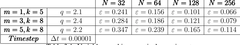
ε=O(N−k/(m+k+2)) = q·N−k/(m+k+2) (3.2) The factorqis determined empirically such that the support widthεis sufficiently wide to get stable converging results. The factor depends on the delta function variablesm

andk. For our numerical tests the values used are summarized below:

NNN = 32= 32= 32 NNN = 64= 64= 64 NNN = 128= 128= 128 NNN = 256= 256= 256

mmm= 1= 1= 1, k, k, k= 5= 5= 5 q= 2.1 ε= 0.241 ε= 0.156 ε = 0.101 ε= 0.066

mmm= 3= 3= 3, k, k, k= 8= 8= 8 q= 2.4 ε= 0.284 ε= 0.186 ε = 0.121 ε= 0.079

mmm= 5= 5= 5, k, k, k= 8= 8= 8 q= 2.2 ε= 0.347 ε= 0.239 ε = 0.165 ε= 0.114

[image:18.612.116.513.630.705.2]

T imestepT imestepT imestep ∆t = 0.00001

(19)

3.2 1D A

DVECTION

E

QUATION

,

TOP

-

HAT

The 1D advection equation with a top-hat initial condition on the domain−1< x < 1 is defined as follows:

∂u ∂t +

1 2

∂u ∂x = 0

u(x,0) = 0 x≤ −0.25

= 1 −0.25< x < 0.25

= 0 x≤0.25

u(−1, t) = 0

(3.3)

The analytical solution is given as:

u=u0(x−1/2t) (3.4)

The initial condition will be filtered using the filter matrix, 2.14:

˜

f0 =Ff0 (3.5)

(20)

3.2.1 Results,

m

= 1

,

k

= 5

[image:20.612.97.523.377.552.2]

(a) (b)

Figure 3.1: Time evolving numerical solution (a) and error (b) for N = 256, m = 1, k = 5,

ε= 0.066

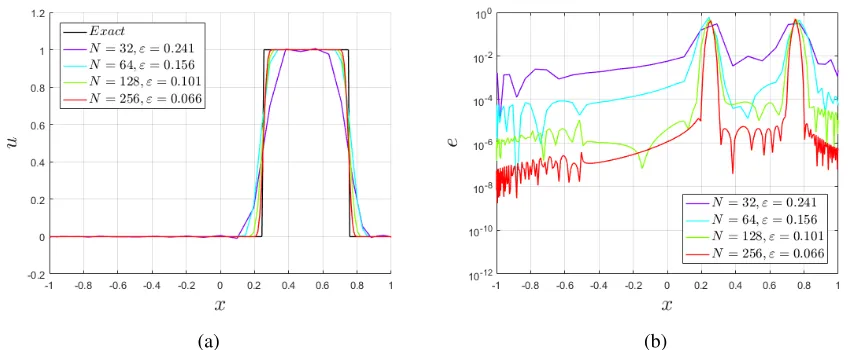
(a) (b)

Figure 3.2: Numerical solution (a) and error (b) att= 1, for the four different grids form= 1,

(21)

3.2.2 Results,

m

= 3

,

k

= 8

(a) (b)

ε= 0.079

(a) (b)

(22)

3.2.3 Results,

m

= 5

,

k

= 8

(a) (b)

ε= 0.114

(a) (b)

(23)

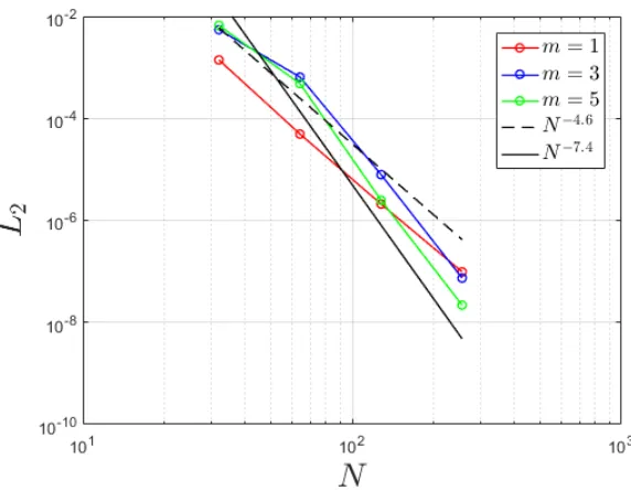
3.2.4 L2 error norm convergence

In order to check the convergence outside the area with the discontinuity, theL2 error

is determined att= 1on the domain−1< x <−0.556for the three different cases. TheL2

error-norm (for the whole domain) is defined as:

L2 =

v u u t

1

N

N X

i=0

(ui,exact−ui,numerical)2 (3.6)

[image:23.612.161.447.285.507.2]

The results are shown in figure 3.7. For reference, lines are plotted to show the order of convergence.

(24)

3.3 1D A

DVECTION

E

QUATION

,

SINUS WITH DISCONTINUITY

The 1D advection equation with a sinus with discontinuity as initial condition on the domain−1< x <1is defined as follows:

∂u ∂t +

∂u ∂x = 0

u(x,0) =sin(πx)−0.5 x≤ −0.25

=sin(πx) + 0.5 x >−0.25

u(−1, t) =sin(π(−1−t))−0.5

(3.7)

The analytical solution is given as:

u=u0(x−t) (3.8)

The initial condition will be filtered using the filter matrix, 2.20:

˜

f0 =Ff0 (3.9)

(25)

3.3.1 Results,

m

= 1

,

k

= 5

[image:25.612.101.522.120.294.2]

(a) (b)

ε= 0.066

(a) (b)

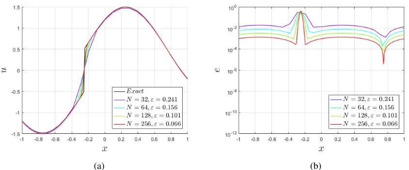
[image:25.612.98.524.376.552.2]

(26)

3.3.2 Results,

m

= 3

,

k

= 8

[image:26.612.101.522.120.295.2]

(a) (b)

Figure 3.10: Time evolving numerical solution (a) and error (b) forN = 256, m = 3, k = 8,

ε= 0.079

(a) (b)

Figure 3.11: Numerical solution (a) and error (b) at t = 1, for the four different grids for

[image:26.612.99.523.376.552.2]

(27)

3.3.3 Results,

m

= 5

,

k

= 8

[image:27.612.100.521.116.294.2]

(a) (b)

Figure 3.12: Time evolving numerical solution (a) and error (b) forN = 256, m = 5, k = 8,

ε= 0.114

(a) (b)

Figure 3.13: Numerical solution (a) and error (b) at t = 1, for the four different grids for

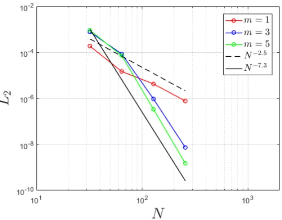
[image:27.612.99.523.377.552.2]

(28)

3.3.4 L2 error norm convergence

is determined att= 1on the domain−1< x <−0.556for the three different cases. TheL2

error-norm (for the whole domain) is defined as:

L2 =

v u u t

1

N

N X

i=0

(ui,exact−ui,numerical)2 (3.10)

[image:28.612.162.445.286.507.2]

The results are shown in figure 3.14. For reference, lines are plotted to show the order of convergence.

Figure 3.14: L2 error norm convergence results for−1 < x < −0.556, sinus w. dicontinuity

(29)

3.4 C

ONCLUSIONS

In this section it is shown that high-order convergence away from the discontinuity can be obtained when filtering discontinuous initial conditions using the filter-matrix.

For the case of the top-hat initial condition the influence ofmon the results is less clear. Higher values ofmseem to show slightly better results, however give a slight over- and undershoot near the discontinuity and require a wider support width to give stable converging results.

In the case of the sinus with discontinuity, the influence ofmis much more clear. Since the regularized delta function is a(m+ 1)th order accurate delta sequence, the error introduced on the smooth parts of the sinus are much lower for higher values ofm. This can best be seen att= 0, which is the filtered initial condition. Since the top-hat consists of straight lines, it does not show this behavior.

(30)

CHAPTER 4 THEORETICAL FILTER-ERROR

4.1 S

MOOTHING OF PIECEWISE FUNCTIONS Given a functionf, letf_εm,k be the function defined by the convolution:

f_εm,k = (f ∗δm,k_ε )(x) = Z x+ε

x−ε

f(τ)δ_εm,k(x−τ)dτ (4.1)

Then in [11], it is proven thatfm,k converges pointwise tof asε→0. Furthermore it is proven that:

f_εm,k(x)−f(x) = O(εm+1) for a+ε < x < b−ε (4.2) We are interested if this convergence is retrieved when filtering a discontinuous signal using the filter-matrix previously defined, equation (2.20).

4.2 C

ONVOLUTION

In the derivation of the filter-matrix, polynomial interpolation is used since the solution is only known on a finite amount of points. To exclude the effect of the polynomial interpolation, first the case of ’pure’ convolution is considered for a sinus with a discontinuity. The signal is given by:

u(x) =sin(πx)−0.5 x≤ −0.25

=sin(πx) + 0.5 x >−0.25

(4.3) The convolution applied to the signalu:

˜

u(x) = Z x+ε

x−ε

u(τ)δ_εm,k(x−τ)dτ (4.4)

(31)

[image:31.612.99.521.77.253.2]

(a) (b)

Figure 4.1: Filtered signal (a) and error (b) for the four different grids,m = 1,k = 5,q = 2.1

(a) (b)

[image:31.612.111.519.323.499.2]

(32)

[image:32.612.161.448.369.588.2]

(a) (b)

TheL2 error results are shown below, for convenience the lines for the theoretical

error convergence and lines to indicate the slope are also plotted.

Figure 4.4:L2error norm convergence results for0.098 < x <0.3827, sinus w. discontinuity

(33)

4.3 P

OLYNOMIAL INTERPOLATION

In the following the polynomial interpolation of the sinus with discontinuity is plotted. Since the filtermatrix basically applies the convolution to the polynomial interpolation of a discrete signal, it is interesting to see the result of this operation. For convenience the expressions for the polynomial interpolation are repeated, [8]:

f(x) = N X

i=0

f(xi)li(x) (4.5)

With

li(x) =ΠNj=0,j6=i

x−xj

xi−xj

(0≤i≤N) (4.6)

The results are shown below.

[image:33.612.100.528.171.529.2]

(a) (b)

(34)

4.4 F

ILTERMATRIX

In the following the error convergence of the (discrete) sinus with discontinuity that is filtered using the filtermatrix, equation (2.20), is considered. The filtered signal simply follows from:

˜

u=Fu (4.7)

Next, the results are shown form= 1/q= 2.1,m= 3/q= 2.4andm= 5/q= 2.2.

[image:34.612.102.520.246.420.2]

(a) (b)

[image:34.612.102.521.489.665.2]

(35)

[image:35.612.99.522.77.253.2]

(a) (b)

TheL2 error results are shown below.

Figure 4.9:L2 error norm convergence results for0.098< x <0.3827, sinus w. dicontinuity

[image:35.612.164.448.350.570.2]

(36)

4.5 F

ILTERMATRIX

,

WIDER SUPPORT

In the following the error convergence of the (discrete) sinus with discontinuity that is filtered using the filtermatrix, equation (2.20), is again considered. However, the support widths are increased.

Below, the results are shown form= 1/q= 2.1,m = 3/q= 3.3andm = 5/q= 3.4.

[image:36.612.113.520.206.378.2]

(a) (b)

Figure 4.10: Filtered signal (a) and error (b) for the four different grids,m = 1,k= 5,q= 2.1

(a) (b)

[image:36.612.112.519.449.624.2]

(37)

[image:37.612.99.521.77.252.2]

(a) (b)

Figure 4.12: Filtered signal (a) and error (b) for the four different grids,m = 5,k= 8,q= 3.4

TheL2 error results are shown below.

Figure 4.13:L2error norm convergence results for0.098< x < 0.3827, sinus w. discontinuity

[image:37.612.164.448.350.570.2]

(38)

4.6 1D

ADVECTION EQUATION

In the 1D advection equation, the initial condition is simply advected with the advection speed, which also follows from the exact solution:

u(x, t) = u0(x−t) (4.8)

In case the initial condition is filtered, as was done in chapter 3, the filtered initial condition will be advected and so will be the error introduced by the filtering. Therefore, intuitively, we expect to retrieve the theoretical filter error convergence,O(εm+1), in the solution of the 1D advection equation as well. In the following this will be proven mathematically.

If we define the linear operatorLas:

L= ∂

∂t + ∂

∂x (4.9)

Then, the 1D advection equation for the unknownucan be written as:

L(u(x, t)) = 0 (4.10) Convolution of this expression with the regularized delta function,δm,k

ε , yields:

Z τ+ε

τ−ε

L(u(τ, t))δ_εm,k(τ−x)dτ = 0 (4.11) SinceLis a linear operator, Leibniz’s rule can be used to takeLout of the integral:

L

Z τ+ε

τ−ε

u(τ, t)δm,k_ε (τ−x)dτ

= 0 (4.12)

The term inside brackets is the filtered version ofu, which we will write asu˜:

(39)

Combining equation (4.10) and equation (4.13) gives:

L(u(x, t))−L(˜u(x, t)) = 0 (4.14)

L(u(x, t)−u˜(x, t)) = 0 (4.15)

L(errorf ilter) = 0 (4.16)

So that the filter error indeed behaves similar to the the solution in the sense that it is also advected. Therefore the error of the 1D advection equation in which the initial condition is filtered will also converge asO(εm+1_).

The foregoing is verified with an example. Consider the problem from section 3.3:

∂u ∂t +

∂u

∂x = 0 (4.17)

u(x,0) =sin(πx)−0.5 x≤0 (4.18)

=sin(πx) + 0.5 x >0 (4.19)

u(−1, t) =sin(π(−1−t))−0.5 (4.20) The initial condition will be filtered using the filtermatrix, equation (2.20). However when using the filtermatrix, the areas near the boundaries of the domain aren’t filtered.

Furthermore the boundary condition isn’t filtered either so that a zero-error enters the domain. This makes it impossible to retrieve the theoretical convergence.

To resolve this, the areas close to the boundaries will be filtered as if the initial condition outside the boundaries were known. This is off coarse not the case in a practical problem, so this is not possible in general. In these areas the filtered initial condition is given as:

˜

u(x,0) = Z x+ε

x−ε

(40)

The problem with the boundary condition is resolved by applying the convolution operation to the boundary condition, yielding a ’filtered’ boundary condition:

˜

u(−1, t) =

Z −1+ε

−1−ε

[sin(π(τ−t))−0.5]δ_εm,k(−1−τ)dτ (4.23) These integrals can again be solved using Clenshaw-Curtis quadrature as was done with the filtermatrix.

Using the aforementioned artificial ’tricks’, the 1D advection equation with a discontinuous sinus as initial condition is solved again to see whether the theoretical filter error is retrieved. The support widths are chosen the same as the ones in section 4.5. For convenience the variables used are summarized below.

NNN = 32= 32= 32 NNN = 64= 64= 64 NNN = 128= 128= 128 NNN = 256= 256= 256

mmm= 1= 1= 1, k, k, k= 5= 5= 5 q= 2.1 ε= 0.241 ε= 0.156 ε = 0.101 ε= 0.066

mmm= 3= 3= 3, k, k, k= 8= 8= 8 q= 3.3 ε= 0.391 ε= 0.255 ε = 0.167 ε= 0.109

mmm= 5= 5= 5, k, k, k= 8= 8= 8 q= 3.4 ε= 0.535 ε= 0.370 ε = 0.256 ε= 0.177

[image:40.612.116.513.309.387.2]

T imestepT imestepT imestep ∆t = 0.00001

(41)

4.6.1 Results,

m

= 1

,

k

= 5

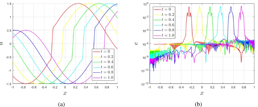
[image:41.612.103.521.119.297.2]

(a) (b)

Figure 4.14: Time evolving numerical solution (a) and error (b) for,N = 256,m = 1,k = 5,

q= 2.1andε = 0.066

(a) (b)

Figure 4.15: Numerical solution (a) and error (b) fort= 1for the four different grids,m = 1,

[image:41.612.108.519.380.555.2]

(42)

4.6.2 Results,

m

= 3

,

k

= 8

[image:42.612.101.520.116.295.2]

(a) (b)

q= 3.3andε = 0.109

(a) (b)

[image:42.612.102.520.380.555.2]

(43)

4.6.3 Results,

m

= 5

,

k

= 8

[image:43.612.101.521.115.294.2]

(a) (b)

q= 3.4andε = 0.177

(a) (b)

[image:43.612.102.518.397.573.2]

(44)

4.6.4 L2 error norm convergence

[image:44.612.163.448.174.394.2]

is determined att= 1on the domain−1< x <0.2903for the three different cases. TheL2 error results are shown below.

Figure 4.20:L2 error norm convergence results for−1< x < 0.2903, sinus w. discontinuity

From the previous plot it follows that the theoretical error convergenceO(εm+1)is indeed retrieved as would be expected.

4.7 C

ONCLUSIONS

In section 4.2 it is shown that the error of a signal that is convoluted with the regularized delta function, converges according to the theoretical filter error.

Then in section 4.3, section 4.4 and section 4.5 it is shown that this is also the case when the polynomial interpolation of the signal is convoluted with the regularized delta function, i.e. using the filter matrix with sufficiently wide support widths to suppress the influence of the polynomial interpolation.

(45)

CHAPTER 5 CONCLUSIONS AND FUTURE WORK

In this present research, the high-order Dirac-delta function presented in [11] is used to smoothen discontinuous initial conditions for the one-dimensional advection equation that is solved using the spectral collocation method. The filtering is based on convolution of the polynomial interpolation of the initial condition with the regularized Dirac-delta function. This operation is written as a matrix vector multiplication using a so-called filter-matrix.

The one-dimensional advection equation is solved for two different filtered initial conditions using different variables for the Dirac-delta function. High-order convergence is found outside the regularization zone. Higher values ofmgive higher convergence especially for the case of the sinus with discontinuity, however they require a wider support width to yield stable converging results.

Finally, the error is compared with the theoretical error. It is shown that in the case of a sufficiently wide support width and filtered boundary conditions, the theoretical value is retrieved.

For future work it is suggested that the application of filtering based on the

(46)

BIBLIOGRAPHY

[1] Clenshaw curtis quadrature. Wikipedia, https://en.wikipedia.org/wiki/Clenshaw-Curtis quadrature, accessed March 2016.

[2] Richtmyer-meshkov instability. Wikipedia,

https://en.wikipedia.org/wiki/Richtmyer-Meshkov instability, accessed September 2016. [3] High order regularization of dirac-delta sources in two space dimensions. Internship

report, Wouter de Vries March 2015.

[4] G. JACOBS ANDW.-S. DON,A high-order weno-z finite difference scheme based particle-source-in-cell method for computation of particle-laden flows with shocks, J. Comput. Phys., 228 (2009), pp. 1365–1379.

[5] S. G. JANHESTHAVEN AND D. GOTTLIEB,Spectral Methods for Time-Dependent Problems, Cambridge University Press, Cambridge, United Kingdom.

[6] J. JUNG,A note on the spectral collocation approximation of some differential equations with singular source terms, J. Sci. Comput., 39 (2009), pp. 49–66.

[7] J. JUNG. AND W.-S. DON,Collocation methods for hyperbolic partial differential equations with singular sources, Adv. Appl. Math. Mech., 1 (2009), pp. 769–780.

[8] D. KINCAID ANDW. CHENEY,Numerical Analysis, Mathematics of Scientific Computing, Brooks/Cole Publishing Company, Pacific Grove, California, 1991.

[9] R. J. LEVEQUE,Finite-Volume Methods for Hyperbolic Problems, Cambridge University Press, Cambridge, United Kingdom, 2004.

[10] C. SEGAL,The scramjet engine; processes and characteristics, University of Cambridge, Cambridge, 2009.

[11] J. P. S. SOLANO,Regularization of Singular Sources for PSIC Computations of Particle-Laden Flows with Shocks, PhD thesis, San Diego State University, San Diego, CA, 2015.

Regularizing discontinuities based on filtering using dirac delta kernels