Dynamic detection of mobile malware using real life data and machine learning

(1)

(2)

August 2018

Master Business Information Technology Track: Data Science & Business

Faculty of Electrical Engineering, Mathematics and Computer Science University of Twente

A

UTHOR

J.S. PANMAN DEWIT

G

RADUATION

C

OMMITTEE

Dr. J.VAN DERHAM

Faculty EEMCS, University of Twente

Dr. D. BUCUR

Faculty EEMCS, University of Twente

Prof. Dr. M. JUNGER

Faculty BMS, University of Twente

S. STEENSMA, MSc. Capgemini NL

CREDITS COVER PHOTO:

Original picture created by Rawpixel.com - Freepik.com Screen image created by Freepik

CREDITSLATEXTEMPLATE:

(3)

i

Abstract

Mobile malwares are malicious programs that target mobile devices, which are an increasing problem. This is reflected by the rise of detected mobile malware samples per year. Addition-ally, the number of active smartphone users is expected to grow, stressing the importance of research on the detection of mobile malware.

Detection methods for mobile malware exists, although methods are still limited and incomprehensive. In this paper, we propose detection methods that use device information such as the CPU usage, battery usage, and memory usage for the detection of 10 subtypes of Mobile Trojans. The focus of this paper is the Android Operating System (OS) as it is dominating the mobile device industry with an 80 per cent market share.

(4)

(5)

iii

Acknowledgements

This thesis could not have been completed without the contribution and help of multiple persons.

First of all I would like to share my appreciation for my supervisors Dr. J. van der Ham, Dr. D. Bucur, and Prof. Dr. M. Junger for their outstanding guidance throughout my thesis process. Their contribution was crucial in improving the quality of this thesis. Additionally, I would like to thank Prof. Dr. L. Cavallaro from the Royal Holloway University of London. He was not part of the graduation committee nor part of the University of Twente. Nevertheless, he was open to share his expertise on mobile security through multiple Skype sessions. These sessions helped improve the quality of this thesis.

Furthermore, I owe a lot of thanks to Capgemini which provided me both with a working place and many interesting people to discuss my findings with. My special thanks goes out to S. Steensma, who has guided me within Capgemini and helped me to focus on the right matters throughout the process of working on my thesis.

Moreover, I would like to thank the Ben-Gurion University, that provided me with the dataset used in this research.

Lastly, I would like to thank my family for their support the past 10 months.

Sebastian Panman de Wit

(6)

(7)

v

Introduction

Nowadays smartphones have become an integral part of life, with people using their phone in both their private and professional life. There is an estimated of 2.6 billion active smartphone users globally at the time of writing, and this number is expected to grow by one billion by 2020 [1]. The rise in smartphone users has also led to an increase in malicious programs targeting mobile devices, i.e. mobile malware. Criminals try to exploit vulnerabilities on smartphones of other people for their own purposes. Additionally, over the past years malware authors have become less recreational-driven and more profit-driven as they are actively searching for sensitive, personal, and enterprise information [2].

Academic work is mainly divided into dynamic analysis and static analysis of mobile malware. Dynamic analysis refers to the analysis of malware during run-time, i.e. while the application is running. Static analysis refers to the analysis of malware outside run-time, e.g. by analysing the installation package of a malware. Dynamic analysis has advantages over static analysis but methods are still imperfect, ineffective, and incomprehensive [3]. An important limitation is that most studies developed malware detection methods based on analysis in virtual environments, e.g. analysis on a PC, instead of real mobile devices. An increasing trend is seen in malware that use techniques to avoid detection in virtual environments, thereby making methods based on analysis in virtual environments less effective than methods based on analysis on real devices [2]. Moreover, we found that most methods are assessed with i) malware running isolated in an emulator, and ii) malware running for a brief period. This kind of assessment does not reflect the circumstances of a real device with for example different applications running at the same time. Therefore, most research does not provide a realistic assessment of detection performances of their detection methods due to their unrealistic circumstances.

(12)

1.1 Research questions

This research uses the following main research question to address the current limitations of dynamic detection methods:

M.Q. 1 How can we improve the dynamic detection of Mobile Trojans using hardware and software features (not requiring any root permissions), based on real-life data?

The main research question is formulated based on an extensive literature research which is described in Sections 2.4 and 2.5. The findings of the literature research lead to the following four focus areas: i) dynamic detection ii) Mobile Trojans, iii) hardware and software features, features not requiring any root permissions, and iv) real-life data. The focus on dynamic detection is chosen because of its advantages over static analysis, which are described in Section 2.4.1. Mobile Trojans are the most prevalent malware type on Android devices and is therefore chosen; more on this can be found in Section 2.1.1. Hardware features and software features, not requiring any root permissions, are chosen because these features are present in the dataset used in this research. Additionally, as stated in the introduction of this Section, focusing on features not requiring any root permissions allows the detection methods of this research to be used on the majority of Android devices. Lastly, the focus on real-life data allows for i) realistic assessment of detection methods and ii) valuable insights on detecting mobile malware on real devices.

The following sub-questions are formulated to help answer the main research question:

S.Q. 1 How do different machine learning techniques such as Random Forest, K-Nearest Neighbour, Naïve Bayes, and Multilayer Perceptrons, perform in detecting Mobile Trojans?

The Random Forest, K-Nearest Neighbour, and Naive Bayes classifiers showed the most promising results in the literature that was consulted for this research. Neural networks, though scantily researched for the detection of mobile malware, show promising results[7]. Therefore, Neural Networks will be examined in this research together with the aforestated classifiers. Related works on dynamic mobile malware detection and the performances of the classifiers in these works can be found In Section 2.5. The answer to S.Q.1 is described in Chapter 6.

S.Q. 2 What software and/or hardware features, that do not require root permissions, are the most crucial for the detection of Mobile Trojans?

Mobile devices are limited in resources such as battery, CPU, and RAM capacity. Therefore examining which features are the most crucial in the detection of mobile malware, and which features can be excluded, improves the efficiency of the detection models. Additionally, the answer to this sub-question provides insights in which features are important in the detection of different subtypes of Mobile Trojans. Because these feature insights are drawn from real-life data, the findings reflect real-life circumstances rather than (clean) laboratory environments. The answer to S.Q.2 is described in Section 6.

S.Q. 3 What is the usability of these different classifiers on a real device?

(13)

1.2. Research method and report structure 3

1.2 Research method and report structure

A research method is devised to answer the research questions in a structured manner. This research methodology is based on CRISP-DM, a widely used data science methodology [8]. This paper is organized according to the research methodology shown in Figure 1.1. The research methodology and the report structure is described below.

Data

preparation Modelling

Results analysis

Usability analysis Domain

understanding understandingData

FIGURE1.1: Research methodology

Domain understanding

This phase is needed to understand the domain of mobile malware. Relevant literature on mobile malware detection is found during this phase. Additionally, the impact of mobile malware on businesses is analysed. Furthermore, recent industry developments in mobile malware detection methods are examined. Chapter 2 contains the findings of this phase.

Data understanding

The dataset used in this research is provided by an external party. Therefore this phase is required to understand the content of the dataset provided. The dataset content is explored with the use of multiple visualisations such as histograms. This phase also consists of verifying the data quality. Chapter 3 contains the findings of this phase.

Data preparation

Multiple preparation steps are needed to construct a dataset that can be used for the creation of detection models. Chapter 4 describe the steps taken during this phase.

Modelling

This phase consists of selecting machine learning techniques, setting up experiments, and training and testing of the machine learning techniques. Chapter 5 describes the steps taken during this phase.

Results analysis

The results of the experiments and feature analysis are collected and documented during this phase. This phase presents the results needed to answer the sub-questionsS.Q.1andS.Q.2. Chapter 6 contains the findings of this phase.

Usability analysis

This phase consists of analysing the usability of the detection models. The usability of de-tection models on real devices is analysed, using multiple metrics such as the training and testing times of classifiers. Additionally, the business usability of the detection models is examined with a cost-benefit analysis. This phase results in the answer toS.Q.3. Chapter 7 describes the findings of this phase.

(14)

(15)

5

Chapter 2

Background

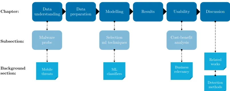
Each subsection of this chapter describes the necessary background knowledge for a specific subsection of this thesis, to understand its content. The related subsections are shown in Figure 2.1.

Data understanding

Data

preparation Modelling Results Usability

Mobile threats

Chapter:

Subsection:

Background section:

Malware probe

Selection ml techniques

ML classifiers

Cost-benefit analysis

Business relevancy

Related works

Discussion

Detection methods

FIGURE2.1: Background chapter overview

2.1 Mobile threats

Mobile malware differs from traditional (PC) malware. Below, the most relevant differences are listed based on [2].

• Mobile devices cross physical and network domains exposing them to more malware such as mobile worms. This kind of malware uses the physical movement of devices in order to propagate across networks.

• Most mobile devices have high application turnover due to the high availability of apps. • The input methods of mobile devices increase the complexity of analysis. Touch com-mands such as swiping and tapping allow for more different input comcom-mands than the traditional mouse and keyboard input. This complicates the analysis of all possible input commands.

• Mobile devices are resource limited with for example a limited battery, CPU, and RAM capacity.

• Mobile devices are susceptible to a wide array of vulnerabilities due to their different ways of connecting to the outside world and the different types of technologies they use. Different connection methods such as Wifi, GPRS, 3G, Bluetooth, make the device more vulnerable. Additionally, the different technologies such as the camera, speaker, make the mobile device more susceptible to vulnerabilities through for example the drivers of these technologies.

[image:15.595.84.487.266.426.2]

(16)

2.1.1 Mobile malware types

To categorize the different mobile malware threats, this research uses the malware type classi-fication of Google [9], shown in Table 2.1. This Table shows only the malware types examined in this research.

Malware type Malicious behaviour description

Trojan Appears benign but performs malicious activity without user’s knowledge. Adware Shows advertisements to the user in an unexpected manner, e.g. on the home screen. Denial of service (DOS) Executes, or is part of, a cyber-attack (DOS attack) without user’s knowledge. Hostile downloader Not malicious itself but downloads malware.

Phishing Appears trustworthy and requests user authentication credentials, but sends the data to a third party. Privilege escalation Breaks the application sandbox or changes access to core security-related features, therefore _{compromising the integrity of the system.}

Ransomware Takes partial or complete control of system and/or data and asks for a payment to release control _{and/or data.} Spyware Transmits sensitive data off the device.

*The adware type is not included in the Google classification as it ‘does not put the device at risk’[6]. This research however, does include this type because adware performs

unwanted behaviour on a device and is therefore malicious. TABLE2.1: Malware classification

The actual distribution of the different types of malware is hard to estimate as detection numbers of Antivirus (AV) vendors rather reflect the efficacy of its detection methods than the actual distribution. However, using different sources helps in giving an impression of the Android malware ecosystem. Figure 2.2 shows the distribution of different types of malware according to the latest security report of Google [9] (left) and of the latest security report by Kaspersky [10] (right). Although Kaspersky uses a different terminology, both figures show the Trojan type being the most common malware. Note that malware types are not mutually exclusive.

Trojan Toll fraudSMS fraud Hostile downloader

Spyware Other

Type

0% 5% 10% 15% 20%

Percentage of malware samples

Google

Trojan.RansomAdwareTrojanTrojan.SMSTrojan.DropperTrojan.SpyTrojan.BankerBackdoor Other

Type

Percentage of malware samples

Kaspersky

FIGURE2.2: Malware type distribution according to Google [9] (left) and Kasper-sky [10] (right)

2.1.2 Android security

(17)

2.2. Machine learning classifiers 7

2.2 Machine learning classifiers

The definition for machine learning used throughout this research is: “the complex compu-tation process of automatic pattern recognition and intelligent decision making based on training sample data” [11]. A more general definition of machine learning is “the process of applying a computing-based resource to implement learning algorithms” [11]. Based on different books on machine learning [11][12][13][14], the basic theory of the different Machine Learning techniques used in this research is described in this section.

Three categories of learning algorithms are: supervised learning, unsupervised learning, and semi-supervised learning. In supervised learning, the goal is to create a model which predictsybased on somex, given a training set consisting of examples pairs of(xi,yi). Here

yiis called the label of the examplexi. Whenyis continuous, the problem at hand is called

a regression problem, and whenyis discrete the problem at hand is called a classification problem. Throughout this research, the focus is on supervised learning as we try to detect whether a device described by some featuresx, contains malware that is performing malicious actions. In this case, the prediction valuey takes the value 1 if a malicious application is performing malicious actions on the device and 0 if no malicious actions are performed on the device. The next Section describe the machine learning classifiers used in this research. Then Section 2.2.6 describes the metrics used to evaluate classifiers. Lastly, Section 2.2.7 describes the challenges of using machine learning to create mobile malware detection methods.

2.2.1 Random Forest

x1

x2 x3

x4 x5

B M B M

x7

B M

x6

B M

< 1 > 1

< 2 > 2 < 4 > 4

< 1 > 1 < 4 > 4 < 2 > 2 < 3 > 3

FIGURE2.3: Example of Decision Tree

The Random Forest (RF) classifier is an ensemble classifier that uses multiple decision tree classi-fiers to classify test instances. An example of a decision tree is shown in Figure 2.3.

A major disadvantage of decision trees is their instability. Decision trees are known for high variance and often a small change in the data can cause a large change in the final tree. Ran-dom Forests try to reduce the variance of decision trees by taking multiple decision tree classifiers to classify testing instances. Then, classification is done using a majority vote among all the

deci-sion trees. Some advantages of Random Forest are i) it overcomes overfitting ii) it can deal with high-dimensional data. Disadvantages include i) accuracy depends on the number of trees ii) it is sensitive to an imbalanced dataset [3].

2.2.2 Naïve Bayes

Naïve Bayes (NB) is a statistical classifier that uses Bayes’s theorem to predict the probability of given query instance belonging to a certain class. Bayes’s theorem, also called Bayes’s rule, calculates the probability of a hypothesisHbeing true, given some evidencee, according to the following formula:

P(H|e) = P(e|H)∗P(H) P(e)

where

P(H|e)denotes the posterior probability ofH, conditioned one P(e|H)denotes the posterior probability ofeconditioned onH P(H)denotes the prior probability ofH

P(e)denotes the prior probability ofe

(18)

ii) insensitive to irrelevant feature data iii) simple and mature algorithm. A disadvantage is that it requires the assumption of independence of features [3].

2.2.3 K-Nearest Neighbour

x₁

x2

C1= M

C2= B

FIGURE2.4: Example of K-Nearest Neighbour Classification

The K-nearest neighbour (KNN) is a distance-based clas-sifier. Distance-based classifiers generalise from training data to unseen data by looking at similarities between training instances. Given a query instanceq, the classifier finds thek training instances, the closest in distance to the query instanceq. Subsequently, it classifies the query instance using a majority vote among thekneighbours. The distance from the query instance to its training in-stances can be calculated using different metrics such as the Euclidean distance, Minkowski distance, or Manhatten distance. An example of the k-nearest neighbour classifi-cation is given in Figure 2.4.

Advantages of KNN are [3]: i) high precision and ac-curacy ii) non-linear classification iii) no assumption of features. The disadvantages are i) it is sensitive to unbal-anced sample set, ii) it is computational expensive.

2.2.4 Artificial neural networks

M

B

Hidden Layer

Input Layer Output Layer

w1 51

w2 41

x1

x2

x3

x4

w1 61

w1 74

w2 97

FIGURE2.5: Example of an Artificial Neural Network

Artificial neural networks (ANN) is a machine-learning model that uses a structure of nodes, i.e. artificial neurons, to classify testing instances. These nodes are connected to each other by di-rected links. An ANN consists of an input layer, some hidden layers, and an output layer. Every directed link between neurons has some numeric weight shown aswijin the example ANN, shown in Figure 2.5. These numeric weights are used in the activation function of each node. This ac-tivation function is used to determine the output of a node. Different learning algorithms can be used to determine the number of hidden layers,

the number of neurons, and the weights between the neurons. Some of the most popular are feed-forward back-propagation and radial basis function networks. This research uses the Multilayer Perceptron (MLP) classifier which is a class of ANN that uses backpropagation for learning.

2.2.5 AdaBoost

(19)

2.2. Machine learning classifiers 9

2.2.6 Evaluation classifiers

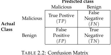
Different performance metrics exist to evaluate a classifier. The most basic performance metrics are summarized in a confusion matrix. The design of a confusion matrix is shown in Table 2.2.

Predicted class

Malicious Benign

Actual Class

Malicious True Postive₍

TP)

False Negative

(FN)

Benign

False Positive

(FP)

True Negative

(TN)

TABLE2.2: Confusion Matrix

The confusion matrix shows how many malware instances were correctly classified as being malware(TP), how many malware instances were missed (FP), how many benign instances were correctly classified as being benign(TN), and how many benign classes were incorrectly classified(FN).

Other metrics and their formula are shown in Table 2.3. These metrics use the metrics shown in Table 2.2. A frequently used metric is the accuracy of a malware, defined by the percentage of correct predictions(TP+TN), of the total predictions(TP+TN+FP+FN). This metric, however, might not reflect the performance of a classifier well. In a skewed dataset, that is a dataset containing more of one class than the other, high accuracy can be achieved by always predicting the majority class. For example in a dataset consisting of 90% malicious actions and 10% benign actions, always predicting malicious actions results in an accuracy of 90%. In the case of a skewed dataset, the performance metrics Precision (PPV) and/or Recall (TPR), reflect the performance of a classifier more realistic. The harmonic mean of the Precision and Recall are reflected in the f1 score (F-score withα=1).

Metric Formula

Accuracy _TP₊TP_TN+₊TN_FP₊_FN

True Positive Rate (TPR) _TPTP₊_FN

False Positive Rate (FPR) FP

FP+TN

True Negative Rate (TNR) _TNTN₊_FP

Precision (PPV) _TPTP₊_FP

F-score (F-measure) (1+α2)( PPV∗TPR

α2(PPV+TPR)) TABLE2.3: Performance Metrics

2.2.7 Automated detection

Two relevant challenges of using machine learning to create mobile malware detection meth-ods are: i) the use of imbalanced datasets and ii) concept drift. Both concepts are described below.

Imbalanced dataset

[image:19.595.191.384.145.240.2]

(20)

Concept drift

The inability of detection models, trained on older malware, to detect new rapid evolving malware, is called concept drift [15]. A way to overcome this issue is to continuously retrain the models, based on new information.

2.3 Business relevancy

The increasing adoption of mobile devices in the workplace, rise in mobile cyber attacks on businesses, and recent legislation, show that mobile security in the workplace is becoming more relevant for businesses. These developments are described in more detail below.

1. Increasing adoption of mobile devices in the workplace:

A recent industry study on the adoption of mobile devices in the workplace shows that nearly 80% of the employees are using a mobile device for business purposes [16].

2. Rise in mobile cyber attacks on businesses:

A recent industry study surveying 588 IT security professionals from the Global 200 compa-nies in the U.S. report that 67 per cent of the respondents said it was certain or likely that their organization had a data breach as a result of a mobile device used by an employee [17]. Another study from a cybersecurity company securing 500 devices of 850 organization show that 100 per cent of the organization experienced at least one mobile malware attack from July 2016 to July 2017.

3. Increased legislation on personal data protection:

A recent development increasing the importance of mobile security in the workplace is the recent General Data Protection Regulation (GDPR), enforced since May 25, 2018. This regula-tion controls the "processing by an individual, a company or an organisaregula-tion of personal data relating to individuals in the EU" [18]. A recent study by Gartner predicts that by 2019, 30 per cent of organizations will face "significant financial exposure from regulatory bodies due to their failure to comply with GDPR requirements to protect personal data on mobile devices" [19][20].

To view how the detection methods in this research fit with the cybersecurity-related activities of business, the cybersecurity framework of The National Institute of Standards and Tech-nology (NIST) [21] is used (shown in Figure 2.6). This framework help businesses manage cybersecurity-related risks. In this Section the framework is used to show in which activities, the detection methods of this research provide business value. Section 7.2 then describes a cost-benefit analysis of the created detection models from a business perspective.

•Recovery planning •Improvements •Communication

•Asset Control •Awareness •Data security

•Information Protection Processes •Maintenance

•Protective technology

•Anomalies and events •Security continious Monitoring •Detection processes •Response planning

•Communication •Analysis •Mitigation •Improvements

•Asset management •Business environment •Governance •Risk Asessment •Risk Management

Strategy

Cybersecurity Framework

Recover Protect

Respond Detect

Identify

FIGURE2.6: NIST Cybersecurity framework

(21)

2.4. Mobile malware detection methods 11

and is not concerned with any of the other categories such as the protection, or recovering of mobile malware threats.

2.4 Mobile malware detection methods

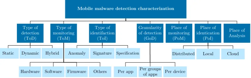
There are numerous ways to detect mobile malware on smartphones. The taxonomy used in this research is a combination of the taxonomy of [3] and [22], and shown in Figure 2.7.

Mobile malware detection characterization

Type of detection (ToD)

Type of monitoring

(ToM)

Type of identifaction

(ToI)

Granularity of detection

(GoD)

Place of monitoring

(PoM)

Place of identication

(PoI)

Place of Analysis

Static Dynamic

Hardware Hybrid

Software Firmware Others

Anomaly Signature Specification

Per app Per groups _{of apps} Per device

Distributed Local Cloud

FIGURE2.7: Mobile malware detection taxonomy

Figure 2.7 shows that detection methods are classified depending on the way the methods are designed. Below, the characterizations of the detection methods and their brief description is described.

Characterization Description

Type of detection The approach taken to collect features by the detection method. Type of monitoring The features being monitored / analysed by the detection method. Type of identification The way malware is identified by the detection method.

Granularity of detection How fine or coarse, data is being analysed by the detection method. Place of monitoring

Where the different steps of the detection method take place. Place of identifcation

Place of analysis

TABLE2.4: Mobile malware detection characterization description

2.4.1 Type of detection

[image:21.595.89.489.193.318.2]

(22)

2.4.2 Type of monitoring

The type of monitoring is defined by the features used within a mobile malware detection method. These features act as an input to the analysis of the detection method. Features can be categorized into three classes: i) hardware, ii) software, and iii) firmware. Hardware features are features that can be monitored and are specific to a device, e.g. battery, CPU, and memory features. Software features are characteristics that can be monitored during the run-time of software or by examining the software package, e.g. permissions, privileges, and network traffic. Firmware features are features from programs using read-only memory. Most firmware features require rooting privileges in the Android OS.

Table 2.5 shows an overview regarding the features used in dynamic mobile malware detec-tion methods. This table is made using a recent literature review on dynamic mobile malware detection methods [3] and was consulted during the preliminary literature research of this research. During the preliminary literature research, few articles were found that focused on hardware features. Therefore, additional literature was searched on detection methods using hardware features. These articles are described in Section 2.5.

Category Feature Papers

Hardware Battery [23], [24], [25]

CPU [23], [24], [26]

Memory [23], [24], [26]

Software Permissions [24], [26], [27], [28], [29], [30], [31] Network Traffic [32], [33], [34], [35]

Information Flow [36], [37] Covert Channel [38]

Firmware System Calls [24], [28], [39], [40], [41], [42], [43], [44], [45], [46]

API [28], [31], [39], [43], [47]

Library [48]

Others Irrelevant Bad terms [49]

Topology Graph [50] Run-time behavior [30], [45]

TABLE2.5: Dynamic detection feature usage overview

2.4.3 Type of identification

The detection methods can also be characterized on the principle which guides the identifica-tion.

Signature-based detection

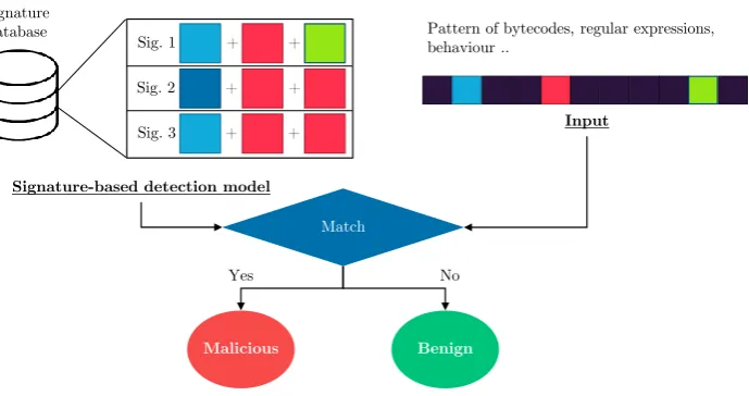
This type of detection, also known as misuse-based detection, uses signatures to identify malware. In static detection, these signatures can be, for example, binary patterns or snippets from software code. In dynamic detection, these signatures can be a pattern of behaviour. Known malware is used to extract patterns, and to form signatures for detection. Then these known signatures are used to detect malware. This type of detection is especially useful for known malware but less effective against zero day-attacks [3]. The process of signature-based detection method is shown in Figure 2.8. This figure illustrates an example of a signature-based detection model that uses snippets from software code as signatures.

(23)

2.4. Mobile malware detection methods 13

Signature database

Sig. 1

Sig. 2

Sig. 3

+ +

Signature-based detection model

Pattern of bytecodes, regular expressions, behaviour ..

Input

Match

Yes No

Malicious Benign

FIGURE2.8: Signature-based detection method

in this case by changing the software code, therefore changing the signature of the app [2].

Anomaly-based detection

This type of detection is based around normal and anomalous behaviour. The former being behaviour which falls within the usual behaviour and the latter being behaviour differing from the normal behaviour. This type of detection is suitable for detecting zero day-attacks, however, they are also prone to false positives. Rare legitimate behaviour can be viewed as malicious by this type of detection. The process of anomaly-based detection method is shown in Figure 2.9

Normal Profile Input

Anomaly?

Yes No

FIGURE2.9: Anomaly-based detection method

Figure 2.9 shows that the detection method needs a profile of normal behaviour. Using this profile, the detection method checks whether any input is similar to this normal behaviour. In the figure, the normal behaviour is shown in a graph as some function over time. This graph can, for example, represent the CPU usage over time. In this case, the normal behaviour shows that CPU usage gradually declines and increases over time. The input, shown on the right in the figure, shows that the CPU usage has a spike. If this spike is higher than some given threshold, the input is flagged as an anomaly.

Specification-based detection

[image:23.595.119.464.75.257.2]

(24)

Rule set for apps Input Rule 1: Allowed to turn on Camera

Rule 2: Allowed to take picture Rule 3: Allowed to access SD-Card

Action 1: Opens Camera Action 2: Takes picture Action 3: Accesses the Internet

App

Allowed?

No Yes

FIGURE2.10: Specification-based detection method

In Figure 2.10, a rule set of three rules is used as an example. These three rules are actions allowed by applications. In this example, applications can turn on the camera, take a picture, and access the SD-card. This can be an example of a simple Camera app. The input comes in the form of actions. Assuming that the three rules in the rule set are the only ones defined, the input in Figure 2.10 would be flagged as malicious. This is because the first two actions in this example are allowed but the third action is not.

2.4.4 Granularity of detection

This categorization refers to the approach taken to handle the collected data during analysis. Malware detection methods can treat data from different applications separately (per app), per groups of apps, or per device. When the malware is a stand-alone application, treating the data per app results in good performance. However when malware is distributed and malicious activity is performed using multiple apps, treating the data per group of apps is more useful. Lastly, for certain types of malware such as rootkits, it could be useful to monitor the device as a whole.

2.4.5 Place of monitoring, identification and analysis

The place of monitoring, identification and analysis can differ between different malware detection methods. These activities can take place distributed, locally or in the cloud. When any of these activities are done in a distributed manner, multiple (trusted) devices are col-laborating to achieve tasks within that activity. Locally refers to any activity taking place on the device itself. Lastly, the activities can take place in the cloud. Monitoring and analysing malware on phones require lightweight approaches as the resources on most devices are limited. Cloud solutions can help alleviate the aforementioned problem.

(25)

2.5. Related works 15

2.5 Related works

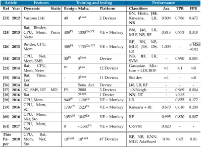
[image:25.595.86.485.221.523.2]

Related papers on dynamic malware detection using hardware features are found using a systematic literature research. The process of the systematical literature research is shown schematically in Appendix B. An overview of the papers found are shown in Table 2.6. This Table includes this paper for comparison. Section 2.5.1 describes the most important findings per paper. Developments in mobile security are examined to augment the knowledge on recent developments in mobile malware detection methods. The industry developments are described in Section2.5.2.

To the best of our knowledge, this research is the first in using data spanning a complete year of +45 real devices for the creation of mobile malware detection methods.

Article Features Training and testing Performance

Ref Year Dynamic Static Benign Malw. Platform Classifiers Acc TPR FPR [53] 2012 Various (14) 40 4Cust _{2 Devices} BN, Histo,

J48,

Kmeans, LR,

NB

0.809 0.786 0.475

[24] 2013

Bat, Binder, CPU, Mem, Netw

Perm 408PS 1330Ge,VT VE + Monkey BN, J48, LR,

MLP, NB, RF 0.813 0.973 0.310

[26] 2013 Binder, CPU,

Mem 408PS 1130Ge, VT VE + Monkey

RF, BN, NB, MLP, J48, DS, LR

1.000

-√

MSE =0.02

[54] 2013 CPU, Net,

Mem, SMS 30PS 5Cust Device

NB, RF, LR,

SVM - 0.990 0.001

[23] 2014 Bat, CPU,

Mem, Netw PS 3Cro 12 Devices

Gaussian

Mix-ture + LDCBOF ≈1 ≈1 ≈0

[55] 2014 Bat, Time,

Loc - 2Cust 11 Devices Std dev ≈1 - ≈0

[56] 2014 Bat Sens. Act. Device J48, LB, RF - -

-[57] 2016 SC, SMS, UP MD PS 2800 3 Devices 1-NNeigh. - 0.969 0.004

[38] 2016 Bat 7Cust 1 Device NN, DT - >0.85

-[58] 2016 CPU, Mem 940PS 1120Ge VE + Monkey LR - 0.855 0.172 [59] 2016 CPU, Mem,

SC 1709PS 1523Dr VE + Monkey Kmeans + RF 0.670 0.610 0.280

[60] 2016 CPU, Mem,

Net, Sto 1059PS 1047Dr VE + Monkey RF 0.995 0.820 0.007

[61] 2017 CPU, Mem,

Net 0 <5560Dr VE + Monkey C-SVM 0.820 -

-This Pa-per 2018 CPU, Bat, Mem, Net, Sto

10Cust ₁₀Cust _{47 Devices} RF, NB, KNN,

MLP, AdaBoost 0.96 0.65 0.01

Batbattery,BNBayesian Network,CrCrowdroid [62],CustCustom,DrDrebin [63],DSDecision Stump,DTDecision Tree,GeMalware Genome Project [64] ,HistoHistogram,KmeansK Means Clus-tering,LDCOFLocal Density Cluster Based Outlier Factor,LocLocation,LRLogistic Regression,Mem memory,MDmetadata,MLPMultiLayerPerceptron,NBNaive Bayes,Netwnetwork,NNNeural Net-work,NNeighbourNearest Neighbour,Permpermissions,PSPlay Store,RFRandom Forest,Std dev Standard Deviation,Stostorage,SVMSupport Vector Machine,SCsystem calls,UPuser presence,

VEVirtual Environment,VSVirusShare[65]VTVirusTotal[66]

TABLE2.6: Related works

2.5.1 Academic works

(26)

Regression, and Naïve Bayes. In the two experiments in which they used the same device for the training and testing of their model, the J48 decision tree classifier performed the best. In the first experiment, all benign and malicious applications were included in the training set, resulting in a TPR of 99% and an FPR of 0%. In this experiment, the training set was 80% of the total dataset and the testing set was 20% of the total dataset. The second experiment did not include all the benign and malicious applications in the training set, leading to a TPR of 91% and an FPR of 11%. In this experiment, the training set contained 3 of the 4 malicious applications and 3 of the 4 benign applications. The remaining malicious application and benign application were used for the testing set. In the two remaining experiments the device on which the model was tested, differed from the training device. For both experiments, the Naïve Bayes classifier performed the best. Including all benign and malicious applications in the training set led to a TPR of 91.3% and an FPR of 14.7%. The training set was created with the all feature vectors from one device. The testing set consisted of all the feature vectors from another device. Not including all the applications in the training set resulted in a TPR of 82.5% and an FPR of 17.8%. In this experiment, the training set consisted of the feature vectors of the 3 malicious applications and 3 benign applications from one device, and the testing test consisted of the feature vectors of the remaining malicious and benign application of another device.

Andromaly showed the potential of detecting malware based on dynamic features using machine learning, compared different classifiers, and used data collected from real devices for the training of its detection model. It also tested its robustness by experimenting with changing the training device from the testing device, and by not including all applications in the training set. The paper, however, is relatively old and much has changed regarding the malware ecosystem since 2012. Furthermore, Andromaly showed promising results but the False Positive Rates of all their four models were relatively high.

In [24], published in 2013, the authors propose a framework named STREAM, which was developed to enable rapid large-scale validation of mobile malware machine learning classifiers. Their framework used 41 features which were collected every 5 seconds from different emulators running in a so-called ATAACK cloud. The feature categories used were Binder, Battery, CPU, Memory, Network, and Permission features. The emulator used the Android Monkey application to simulate pseudo-random user behaviour such as touches on the touchscreen. To evaluate their detection model, the authors used a Random Forest, Naïve Bayes, Multilayer Perceptron, Bayes Network, Logistic Regression, and a J48 classifier. For their training set, they used 408 popular applications from the Google Play Store and 1330 malware applications from the Malware Genome Project database[64], and the VirusTotal database [66]. As the testing set, they used 24 benign applications from the Google Play Store, and 23 malware applications from the Malware Genome Project database, and the VirusTotal database. The best performing classifier was the Bayesian Network which had an accuracy of 81.26% with a TPR of 97.30% and an FPR of 31.03%.

This paper showed the potential of using dynamic features although the FPR for all their tested classifiers were relatively high. Additionally, this research ran applications separately for 90 seconds and made use of a virtual environment in the form of an emulator with user-like behaviour created by the Android Monkey tool. This lowers the confidence that the model would perform the same when evaluated on a real device with a real user.

(27)

Only the performance results are shown for the different Random Forest classifiers with different parameters. The authors used a 5-fold cross validation for the training and testing of their classifiers. The best performing classifier had 160 trees, used 8 different features, and had a tree depth of 16. This resulted in an accuracy of 99.9857% and a root MSE of 0.0183%. Only 2 False Positives were measured during this experiment.

This paper shows the potential of using dynamic features and Random Forest Classifiers. However, as this paper makes use of the dataset by Amos [24] it is sensitive to the same limitations; thus it is not known how this model would perform on a real device with a real user.

In [54], published in 2013, the authors evaluated different machine learning classifiers for their detection model. Their model used 10 features related to memory, network, CPU, and SMS for their detection model. 30 normal applications and five malware applications were used, however, the source of these applications is unmentioned. The malware applications were a Spyware, a Hostile Downloader, a Root1, Spyware, and two Trojan Spyware applica-tions. The benign and malicious applications were run on a real device but it is unknown how and how long the features were collected from these devices. To reduce the size of their feature set, the authors used the Information Gain algorithm. The features left over were related to the Memory, Virtual Memory, SMS, and CPU usage. The classifiers Naïve Bayesian, Logistic Regression, Random Forest, and SVM were evaluated. The training and testing were done with a ten-fold cross-validation. The best performing classifier was the Random Forest classifier with a TPR of above 98.8% for the different families of malware, and an FPR below 1%. This research shows the potential of using dynamic features but due to the lack of description of the feature collection, it is unknown how reliable the performance evaluations are. Additionally, only 5 different malware applications were tested.

In [23], published in 2014, multiple hardware features are taken for the use of anomaly-based detection of mobile malware. The features collected were CPU, memory, battery, amount of connection requests, and ICMP requests. Data from 12 smartphones was collected with the use of an application called Data Collector. These smartphones contained the most popular software in the Android market as benign application and three malware developed by [62] as malware. A Gaussian Mixture Model with a Cluster-Based Local Outlier Factor was used for their detection model. This model resulted in an FPR of almost zero and a TPR of almost 100%. This research shows the potential of using a Gaussian Mixture Model with user behavioural features for the detection of mobile malware, however, no description of the feature collection has been stated. This makes it hard to estimate the reliability of the performance evaluations. Additionally, only three different types of malware were used in this research.

In [25] the authors describe two techniques for detecting malware based on individual power consumption profiles, time, and location. This research has further been refined in [55] where they propose three power-consumption based techniques based on improved data. Both studies show that malware can be detected using power consumption based detection techniques with low False Positive Rates. Their first technique described in [55] uses location-specific power profiles of users. The reasoning behind creating such profiles was that users would be expected to use their device differently depending on their current location, and this would thus lead to different power consumption profiles. The technique was evaluated using over 10 users which ran two simulated malware. The first simulated malware was an SMS Spam malware and the second simulated malware was a Root Spyware. First, location-based power profiles were made for the users with devices not containing any simulated malware. Then by running simulated software and checking for anomalies in the location-based power profiles, the detection model would detect malware on the devices. An anomaly was reported whenever the power consumption would differ a certain amount of sigma outside of the normal power consumption. No complete results were mentioned albeit for the subset of 11 users, using one location, and a sigma of 2.5, a TPR of 100% was achieved with an FPR of 1.5%. The second technique was based on time-based power profiles. With this technique, different power profiles were made depending on the time of the day.

(28)

The reasoning behind this experiment was that users would be expected to use their device differently, and thus having a different power consumption profile, depending on the time of day. In the paper, results for two phones are described where the time profiles are based on blocks of six hours, resulting in four different time periods per day. For a sigma of 2.5%, a TPR of 43.7% and an FPR of 1.7% was achieved. The third technique combines created power profiles based on both location and time. A TPR of 82.7% and an FPR of 1% was achieved, based on results from two users, three different locations, and four different time periods The above-described research shows the potential of using location- and time-based power profiles for the detection of mobile malware. However, results are only shown for a small subset of users, making it hard to determine the actual performance of the detection models. Additionally, only two types of simulated malware were used for the detection model, making it hard to estimate how the detection model would perform on other types of mobile malware.

In [56], published in 2014, the authors examined the possibility of detecting sensitive activities with the use of power consumption measurements. Sensitive activities such as turning the screen on or off, enabling GPS/Wifi, enabling voice recorder, and more where examined. Data was collected using a physical measurement device for the battery level of a real mobile device. The classifiers evaluated were J48, LogitBoost, and Random Forest. No overall performance results are stated but they are given for the Wifi, GPS and Touch classifications. All three classifications had a True Positive Rate of more than 84% with the use of a window size, for the power measurement, of 4000 mSec. The False Positive Rate is not given but the Precision is given. For all classifications, the precision was more than 85% with a window size of 4000 mSec. The research was not focused on detecting specifically malware but the potential of using the power measurement to detect different sensitive activities was shown.

(29)

three different numbers of applications installed. The light usage device contained only 26 native apps, was mostly on standby, and only used for phone calls and text messages. The medium usage device contained 54 applications, used the device normally although no new apps were installed. The high usage device started with 52 applications, installed 91 new apps, and used his phone as often as possible. The framework achieved a TPR of 96% with their framework and a False Positive rate of less than 0.004%. Furthermore, they detected some zero-day attacks which were undetected by multiple Antivirus Software at that time. Additionally, the performance overhead of the used model is low. As the detection model used system calls as a feature, the detection model needed root permissions.

MADAM showed a high TPR and low FPR with low-performance overhead for their frame-work. The performance of their model was assessed on real devices differing the usage intensity over a period of one week, indicating that the performance results reflect real-life circumstances. A factor limiting the applicability of the framework is its requirement for root permissions as System Calls were used as features.

In [38], published in 2016, the authors used artificial intelligence tools to detect malware based on covert channels. This type of malware uses advanced mechanisms to bypass security frameworks and to extract information. A covert channel is created as a communication channel in order for two colluding applications to extract personal information. An example would be that one application called CCSender has access to sensitive data but does not have permissions to send this over a network. Using the covert channel, this application can then send information to another app, named CCReceiver in this example, who does have access to the network. This covert channel is used such that the communication is hidden. The covert channel can take different forms. For example, the CCSender can change the volume settings and the CCReceiver keeps track of any changes in the volume settings. With eight levels of volumes, this results in three bits per iteration of information. Seven self-made android Covert Channel malware applications were used in the research of [38]. Every malware used a different type of covert channel. The channels used in the research were: 1) type of intent, 2) file lock, 3) system load, 4) volume settings, 5) Unix socket discovery, 6) file size, 7) memory load. The detection was based on two levels of energy consumption measurements. First, a high-level energy consumption measurement was used with a modified version of PowerTutor. This application measured the energy consumption per process running on the system. Second, a middle-level energy consumption was used that measured energy consumption based on the current and voltage values stored in the /sys folder. Based on past values of consumptions in a clean system, without malware, a regression model was created to predict future behaviour. Any power consumption deviating disproportionately from this expected behaviour would be classified as anomalous. Additionally, a classification based model was used, using a set of energy-related features. This classification based model used data from the feature set during the presence and absence of colluding applications. To test their detection model the authors made use of Neural Networks and Decision Trees. The detection models were run on two different smartphones, both being in an idle state. The best performing classifier was the classification-based Neural Network. It was able to detect all seven colluding apps with an accuracy of more than 85%. No false positive information was stated.

The paper showed the potential of using battery features for the detection of malware using covert channels. The accuracy, however, was relatively low compared to other malware detection systems. Also, no FPR information was stated making it hard to estimate its real potential. Furthermore, the data was only collected from phones being in an idle-state and with applications running separately, making it hard to estimate the performance results of phones being in use by real users.

(30)

classification algorithm used was linear Logistic Regression with the use of a sliding window technique. For the training set, they used 571 benign applications from the Google Play store, and 727 malware applications from the Genome project. The test set contained 275 benign applications and 304 malware applications. Lastly, they used a validation set of 94 benign applications and 89 previously unseen malware applications. Previously unseen in this case means that the malware applications were neither in the training set nor the testing set. For the creation of the detection model, the window length, the threshold of the number of mal-ware records contained in each window, and the number of checks differed. Their findings show that CPU and memory usage features in combination with Logistic regression and a simple sliding window technique can be used for the detection of malware. However, their best malware detection model, having a TPR of 95.7% of the malware, showed a relatively high false positive rate of around 25%. The detection model having the highest F-measure achieved a TPR 85.5% and an FPR of 17.2%.

This paper showed the potential of using the memory usage and CPU usage as features for the dynamic detection of mobile malware. However, the detection model showed relatively high false positive rates. Furthermore, by using an emulator with the Monkey application it is hard to estimate whether the performance results would be the same on real devices with real user input.

In [59], published in 2016, the researchers used features related to System Calls, Mem-ory usage, and CPU usage. They traced three values for the CPU feature: i) CPU total, ii) CPU user, and iii) CPU kernel. As memory features, they monitored three types of memory consumption: i) memory consumption by the Dalvik Virtual Machine, ii) native memory usage, and iii) total memory usage. Per type of memory consumption, five features were extracted: i) total proportional set size, ii) the shared RAM, iii) the private RAM, iv) the Heap allocation, and iv) the Heap free. Benign apps were downloaded from the Google Play store and malicious applications were collected from the Drebin dataset [63]. The applications were run for 10 minutes in an Android emulator and features were collected every two seconds. The emulator was fed with user-input from the Monkey application. As detection models, they first used a K-means clustering algorithm to cluster apps based on similarity of memory and CPU usage. Then they used a Random Forest Classifier on every cluster that classified the applications based on their System Calls. For the training, they used 1000 benign applications and 1000 malware applications. The best performing model was the classifier with the 7-means clustering algorithm and a Random Forest classifier of 50 trees. It had an accuracy of 67% and an FPR of 28%.

This paper showed the potential of using System Calls, Memory, and CPU features for the detection of malware. However, due to the use of an emulator with the Monkey application, it is unknown whether the performance results would be the same for real devices with real user input. Also, the performance is relatively low compared to other detection methods. Furthermore, this detection method needs root permission as it uses System Calls as features.

(31)

In [61] the authors used Support Vector Machines to create a detection model based on re-source metrics of mobile phone devices. These rere-source metrics (features) were CPU, Memory and Network usage. The features were monitored system-wide and application-specific. They used the Drebin dataset for the malicious applications. It is unknown how many malware applications were included in their research as they took a subset of the Drebin dataset, not mentioning the amount. However, as the Drebin dataset consists of 5560 malware applica-tions, the amount of malware applications used in this research is less than 5560. An emulator was used for the training on of their model. This emulator was fed with simulated user input events from the application Monkey. The classifier used was a C-SVM with a radial basis function kernel. Their detection model achieved an accuracy of 82 per cent. The False Positive rates are unknown but the precision of the model range from 10% to 90% depending on the malware family.

This paper shows the potential of the use of hardware features such as CPU, memory, and network usage. The model performed relatively bad, based on their high FPR, in comparison with the other detection methods. Furthermore, this paper used an emulator with the appli-cation Monkey, making it susceptible to the earlier mentioned limitations of the usage of an emulator.

In summary, it has been shown that using hardware features might be an effective way of detecting malware on mobile devices. The Naive Bayes, K-Nearest Neighbour, and Random Forest classifiers seem the most promising. Most recent papers have based their detection model on emulators and user-like input from the application Monkey making it hard to estimate their performances on real devices with real users. Additionally, most papers have only run the benign and malicious applications for a few minutes meaning that any malware showing malicious behaviour after a few minutes, would not be detected. Furthermore, a limited amount of research has shown high-performance results.

2.5.2 Industry developments

The recent industry developments on mobile malware detection are briefly described in this section to get a complete view of the state of the art of mobile malware detection methods. The focus is on the developments by Google, as this is the developer of the Android software. The statements below are based on the most recent security report of Google [6].

Dynamic Analysis

Google uses different techniques to check whether an application might perform malicious behaviour before this application is allowed to be published in the Google Play store. One technique includes performing a dynamic analysis on the applications. Only from 2016, Google started adding automated event injections to emulate for example user-input. This is what the Monkey application does as well, as mentioned in different papers described in Section 2.5.1. This improvement led to a three-fold increase in the number of apps flagged as potentially malicious. Google runs the applications in virtual environments and attempts to detect anti-cloaking techniques. These anti-cloaking techniques are ways to hinder analysis in virtual environments.

SafetyNet Integration

Google uses SafetyNet to identify apps and other threats throughout the Android ecosystem. SafetyNet uses security information from different devices such as security events, logs, and configurations. In 2014, Google focused on the detection of applications trying to abuse SMS. In 2016 it integrated its data with the Anomaly Correction Engine to focus on rooting applications. Later in 2016, the combination of the ACE and SafetyNet has been used to identify applications that make devices stop working.

Anomaly Correction Engine

(32)

2016 was over 90% according to Google.

Additional Machine Learning researches

In 2016, Google analysed applications based on their installation patterns. Using a semi-supervised machine learning approach, Google tried to automatically group apps based on install patterns. Google described that it used document analysis and clustering techniques to group PHAs. It is unknown which documents were analysed. Using a clustering algorithm it was able to detect new variants of existing PHA families, detect inconsistencies in previous reviews, and suggest classifications for previously unseen apps based on which cluster an application was the closest to.

Other Antivirus solutions

Altough Google describes good performance results, a recent comparison of different An-tivirus solutions shows a low detection rate of malware by Google [69]. Figure 2.11 shows the accuracy of different popular Antivirus solutions. The False Positive Rates of all antivirus solutions is 0%. This figure shows that Google Play Protect has a low accuracy in comparison with the most popular Antivirus solutions. Unfortunately, the inner workings of these differ-ent Antivirus applications are unknown. Furthermore, it is unknown which specific malware applications were used to evaluate the performances of the different Antivirus solutions in Figure 2.11. Research has shown that Antivirus solutions can easily be bypassed by different obfuscation methods [2]. However, this conclusion is based on relatively old research papers from 2012 to 2014. Whether Antivirus solutions are still easily bypassed is unknown to us at the moment of writing.

Norton

BitDefender McAfee Kaspersky Avast Psafe Google Play Protect 8.0

AV vendor

0% 20% 40% 60% 80% 100%

Accuracy

(33)

23

Chapter 3

Data Understanding

This chapter describes the dataset used throughout this research. Figure 3.1 shows the activi-ties and their planned output for the data understanding phase. These activiactivi-ties are described in the following different sections. Section 3.1 describes how the dataset was created and how it was collected. Section 3.2 describes the basic characteristics of the dataset such as the data types and the number of data points. Section 3.3 describes the data exploration phase with tables, charts, and other visualisation tools to better understand the content of the dataset. Section 4.2 describes the data cleansing process.

Data

collection preprocess.Data descriptionData explorationData Data qualityverification

Raw

dataset Readabledataset

Overview dataset content

Dataset statistics

Data quality report Activity:

Output:

FIGURE3.1: Data understanding activities and output

3.1 Data collection

The dataset [5] used throughout this research is provided by the Ben-Gurion University. This dataset was created by providing 50 volunteers with a Samsung Galaxy S5, which contained software to track device metrics, e.g. battery usage, CPU usage, memory usage. The device also contained a self-written malware that simulated different malware types every month and that logs of its actions taken. The dataset thus consists of device metrics data and mal-ware data. A record of the device metrics dataset includes a specific device’s values for its device metrics, the associated sampling timestamp, and an associated userid. A record of the malware dataset includes details of the actions taken by the malware application, the associated sampling timestamp and an associated userid. The volunteers were instructed to use the smartphone as their sole device for at least two years. and they consented to both the device tracking and the installation of the malware application. Additionally, they were instructed to use the malware application at least once every few days for a few minutes. The malware application (a Mobile Trojan) appeared benign although behaved maliciously, hence could be used as a normal app. Section 3.2.1 describes the malware application and its behaviour in more detail.

(34)

2017

Q1 Q2 Q3 Q4

2016

v1 v2 v3 v4 v5 v6 v7 v8 v9 v10 v11 v12

Tracking additional device metrics

+ >

Tracking 30 devices

Malware

+

Added 20 devices Events

Device theft simulation

!

FIGURE3.2: Timeline of dataset creation

3.2 Data description

The dataset is divided into 13 different probes. A probe is a grouping of multiple sensors that shared the same sample interval. For example system metrics, being part of the T4 probe were recorded every 5 seconds and are therefore joined in one probe.

Of the 13 probes, 6 probes are pull probes which recorded sensor data every fixed interval. Of the 13 probes, 7 probes are push probes which recorded sensor data as soon as new information arrived. For example, the SMS probe recorded a new SMS message immediately after the arrival of an SMS message.

The content, number of fields, and a description of the pull probes and push probes are shown respectively in Table 3.3 and Table 3.4.

Probe Sample _interval Content _fieldsNr. Description

T0 24 hrs

Telephone info 15 Information on the current telephony configuration. Hardware info 6 The device’s hardware configuration.

System info 5 Kernel, SDK, baseband, and general information.

T1 60 sec.

Location 15 Location(anonymized via clustering), speed, and accuracy. Cell tower 5 Cell tower ID, type, and reception info.

Device status 14 Brightness, volume levels, orientation, and modes. Wifi scan 4 Identifiers, encryption, frequency, and signal strength. Bluetooth scan 9 Identifiers, device class (type), parameters, and signal strength.

T2 15 sec.

Accelerometer 51

Stats on 800 samples captured 4 seconds at 200Hz. Linear

accelerometer 51

Gryoscope 51 For each respective axis: mean, median, variance. Orientation 9 covariance between axis, middle sample. Rotation vector 12 FFT components and their statistics.

Magnetic field 51 A subset of these features is extracted from the orientation, rotation, and barometer sensors.

Barometer 16

T3 10 sec. Audio 21 Statistics over 5 seconds.

Light 3 Luminosity

T4

(System) 5 sec.

Global app stats 98 Info on CPUs, memory, network traffic, IO interrupts, and WiFi AP Battery 14 Configuration and statistics on power consumption and temperature.

Apps 5 sec. Local app stats 70 For each running application: stats on CPU, memory and network _{traffic, Linux level process information from the system /proc folder.}

Dynamic detection of mobile malware using real life data and machine learning

A

UTHOR

G

RADUATION

C

OMMITTEE

Abstract

Acknowledgements

Contents

Chapter 1

Introduction

1.1

Research questions

1.2

Research method and report structure

Domain understanding

Data understanding

Data preparation

Modelling

Results analysis

Usability analysis

Chapter 2

Background

2.1

Mobile threats

2.1.1

Mobile malware types

Google

Kaspersky

2.1.2

Android security

2.2

Machine learning classifiers

2.2.1

Random Forest

2.2.2

Naïve Bayes

2.2.3

K-Nearest Neighbour

2.2.4

Artificial neural networks

2.2.5

AdaBoost

2.2.6

Evaluation classifiers

2.2.7

Automated detection

2.3

Business relevancy

2.4

Mobile malware detection methods

2.4.1

Type of detection

2.4.2

Type of monitoring

2.4.3

Type of identification

2.4.4

Granularity of detection

2.4.5

Place of monitoring, identification and analysis

2.5

Related works

2.5.1

Academic works

2.5.2

Industry developments

AV vendor

Accuracy

Chapter 3

Data Understanding

3.1

Data collection

2017

2016

3.2

Data description