This content has been downloaded from IOPscience. Please scroll down to see the full text.
Download details:
IP Address: 129.237.129.215
This content was downloaded on 08/12/2014 at 17:28
Please note that terms and conditions apply.
Reversal permanent charge and reversal potential: case studies via classical
Poisson–Nernst–Planck models
View the table of contents for this issue, or go to the journal homepage for more 2015 Nonlinearity 28 103
(http://iopscience.iop.org/0951-7715/28/1/103)
|London Mathematical Society Nonlinearity
Nonlinearity28(2015) 103–127 doi:10.1088/0951-7715/28/1/103
Reversal permanent charge and reversal
potential: case studies via classical
Poisson–Nernst–Planck models
Bob Eisenberg
1, Weishi Liu
2and Hongguo Xu
21Department of Molecular Biophysics and Physiology, Rush Medical Center, Chicago, IL 60612, USA
2Department of Mathematics, University of Kansas, Lawrence, KS 66045, USA E-mail:[email protected],[email protected]@math.ku.edu
Received 10 May 2014, revised 16 September 2014 Accepted for publication 6 November 2014 Published 8 December 2014
Recommended by T J Kaper
Abstract
In this work, we are interested in effects of a simple profile of permanent charges on ionic flows. We determine when a permanent charge produces current reversal. We adopt the classical Poisson–Nernst–Planck (PNP) models of ionic flows for this study. The starting point of our analysis is the recently developed geometric singular perturbation approach for PNP models. Under the setting in the paper for case studies, we are able to identify a single governing equation for the existence and the value of the permanent charge for a current reversal. A number of interesting features are established. The related topic on reversal potential can be viewed as a dual problem and is briefly examined in this work too.
Keywords: electrodiffusion, reversal permanent charge, reversal potential
(Some figures may appear in colour only in the online journal) Mathematics Subject Classification: 34B16, 76Z05, 78A35, 92C35
1. Introduction
almost all biological functions are controlled one way or another by ion channels, just as almost all digital functions are controlled by the channels of field effect transistors.
The study of electrodiffusion is thus an extremely rich area for multidisciplinary research with diverse applications from computer science, through engineering to biology in which mathematics may lend an important hand by generalizing and understanding the principles that allow control of electrodiffusion. For semiconductors and ion channels, permanent charges add an additional component—probably the most important one—to the rich behaviour. A single permanent distribution of charge (i.e., doping) creates several different devices, with robust reduced descriptions, when different electrical potentials are placed on its boundaries, e.g., amplifiers, limiters, multipliers, logarithmic convertors, exponentiators and so on. Permanent charges come into the picture in semiconductors and ion channels in different ways: for semiconductors, one would like to (at least theoretically) design a permanent charge (doping profile) for the semiconductor to achieve a desired performance; for ion channels, one would like to detect (see, e.g., [8–10]) the distribution of permanent charges—a structural property of ion channels—and to analyse its roles in ion channel functions (permeation, selectivity, stability, etc). Synthetic ion channels are now being created ([44], etc) in which the distributions of permanent charge can be created and tested and exploited for technological use.
In this work, we will focus on some basic questions about how permanent charges affect ionic flows; more precisely, we will study when and how a permanent charge produces current reversal using the classical Poisson–Nernst–Planck (PNP) model for ionic flows. It is important to remember that our model is a reduced model with effective parameters that depend on atomic scale details in many ways. In fact, for ion channels, a permanent charge reflects the structure of the channel protein, and its distribution of amino acid side chains, with acidic side chains contributing permanent negative charge and basic side chains contributing permanent positive charge, according to their ionization states, regulated by local pH. Thus, what we call permanent charge density can depend on the location of many atoms, the shape of the protein, etc. Reduced models are needed to compute current–voltage relations of channels in a variety of ionic conditions. As far as we know, all atom simulations cannot deal with the range of concentrations important for biological function, e.g., calcium ions at 10−8M.
1.1. PNP models for ionic flows
There are many models, from low resolution to high, for ionic flows in various settings (see, e.g., [2–4,11,12,16,18,21–24,28–30,35–37,40,41,43,45,46,51–54]). Among them, primitive PNP models have been extensively examined analytically and numerically.
In this work, we take a one-dimensional PNP model. A one-dimensional dimensionless steady-state PNP system forntypes of ion species through ion channels is, fork=1,2,· · ·, n,
ε2 h(x)
d dx
h(x) d
dxφ
= − n
s=1
αscs−Q(x),
dJk
dx =0, −Jk= h(x)Dkck
d dxµk
(1.1)
with the boundary conditions
φ (0)=V0, ck(0)=lk0; φ (1)=0, ck(1)=rk0. (1.2)
Hereε2 1 is a dimensionless parameter,h(x)represents the cross-section area of the ion
channel overx, φ is the electric potential, Q(x)is the permanent charge, and, for the kth ion species,ckis its concentration (number density),αkis its valence (number of charges per
ion flux density,lkandrk are its concentrations at the boundaries (left and right baths). For
boundary conditions, one often imposes the electroneutrality conditions on the concentrations
n
s=1
αsls= n
s=1
αsrs=0. (1.3)
The electrochemical potentialµk(x)for thekth ion species consists of the ideal component
µid
k (x)and the excess componentµ ex k (x):
µk(x)=µidk(x)+µ ex k (x)
where the ideal component is
µidk(x)=αkφ (x)+ ln
ck(x)
c0 (1.4)
with some characteristic number densityc0. Since the only relevant quantity from the chemical
potential lnck(x)
c0 is its gradient, without loss of generality, we will setc0 = 1 in the sequel. The classical PNP model only deals with the ideal componentµid
k(x), which reflects the
collision between ion particles and water molecules and ignores the size of ions. The excess electrochemical potentialµex
k (x)accounts for the finite size effect of ions. This component is
essential for dealing with properties of bulk ionic solutions containing divalents like calcium ions, or mixtures, and is in fact needed whenever concentrations exceed say 50mM, as they almost always do in technological and biological situations. This component is extremely important for many critical properties of ion channels, for example, ideal sodium and potassium solutions are indistinguishable, but life depends on the ability of channels to distinguish between these ions. We refer the readers to, for example, [5–7,47,49,50] for concrete models. In applications, both local models forµexk (x)(a function of the values{cj(x)}atx) and nonlocal
models forµexk (x)(a functional of the functions{cj}) are employed for a variety of purposes.
1.2. An elementary property and a basic question
We will briefly discuss a particular aspect of ionic flows from the model which leads to our question in terms of specific quantities in the model.
Dividingh(x)Dkckthrough the Nernst–Planck equation for the ion fluxJk in (1.1) and
integrating fromx=0 tox=1, one has
Jk
1
0
1
h(x)Dkck(x)
dx=µk(0)−µk(1). (1.5)
Sinceh(x)andck(x)are positive, the sign ofJk is the same as that ofµk(0)−µk(1). For
any local model ofµexk , the latter is completely determined by the boundary values of electric potentialV0and of concentrationslk’s andrk’s; in particular, it isindependentof a permanent
charge. In the language of biologists and chemists, the sign ofJkis determined by the driving
force (the gradient of electrochemical potential) and not the structure (permanent chargeQ) of the channel protein.
For the classical PNP model whereµk(x)= µidk (x) =αkφ (x)+ lnck(x), one has the
explicit formula forµk(0)−µk(1):
Jk
1
0
1
h(x)Dkck(x)
dx=µk(0)−µk(1)=αkV0+ ln
lk
rk
. (1.6)
On the other hand, the actualamountof eachJkdoes depend onQsince the profile of
I. For givenV0,Q(x),lk’s andrk’s, if(φ (x;ε), ck(x;ε), Jk(ε))is a solution of the boundary
value problem (1.1) and (1.2), then the currentIis
I=I(ε)=
n
s=1
αsJs(ε). (1.7)
The electrical current is the important variable for a number of reasons. (1) It is what is almost always measured. (2) Almost all our technology involves electrical currents and potentials. Little involves ion fluxes. (3) Maxwell’s equations can be viewed as the ultimate statement of conservation of charge, a generalization of Kirchhoff’s current law that says current is always exactly conserved no matter how different the carrier of the current (electrons in a cathode ray tube, the displacement current in a vacuum, holes and ‘electrons’ in a semiconductor, ions in an electrolyte solution).
It is important to realize that the components of the current can be positive or negative because of the sign ofαk’s of the charges. Thus the current has much more complexity than
the individual ion fluxes. We are thus interested in how the sign of the current depends on the permanent charge via classical PNP models.
For classical PNP models with the electroneutrality assumption (1.3) and thatDk=1, it
is known (e.g., [4,48] forn =2 and [42] for generaln) that, ifQ=0, thenV0 andIhave
the same sign (independent of the boundary concentrationslk’s andrk’s). Furthermore, as an
immediate consequence of (1.6), one has the simple property below.
Proposition 1.1. If the quantities αk(αkV0 + lnlk − lnrk), for k = 1,2, . . . , n, are all nonnegative (nonpositive), then the quantitiesαkJk’s are all nonnegative (nonpositive), and hence, the currentIis nonnegative (nonpositive) too, independent of a permanent chargeQ; that is, under the above condition onV0,lk’s andrk’s, no permanent chargeQcan reverse the sign of the currentI.
In general, the sign of the currentIcould be reversed. This fact has been used to identify the type (i.e., selectivity) of ion channels in biological experiments since 1949 ([26,27]). A natural question is then:
Question:Under what conditions onV0,lk’s andrk’s, can currentIbe reversed for appropriate choices of permanent chargesQ?
We raise this question from the mathematical analysis point of view, which captures the general physical and biological importance of the issue. The profile of Q in general governs many of the properties of ion channels and semiconductor devices.
A related well-known topic is the reversal potential:for givenQ,lk’s andrk’s, what is the so-called reversal potentialV0 so thatI = 0? Identification of reversal potentials is a
central subject in experiments on channels; indeed, identification of reversal potentials is often a prerequisite for further identification of a channel or transporter.
1.3. Setup of our case study
To this end, we specify the case we will study in this paper. We will examine the question by working on the simplest model,the classical PNP(cPNP) model (1.1) with ideal electrochemical potentialµk=αkφ+ lnck, and the boundary condition (1.2). We will focus
on the case with equal diffusion coefficients (see remark1.1below) and with a simplest profile of a permanent chargeQ. More precisely, we will assume
(A3) A piecewise constant permanent chargeQwith one nonzero region; that is, for a partition
x0=0< x1< x2< x3=1of[0,1],
Q(x)=
0, x ∈(x0, x1)∪(x2, x3)
Q2, x ∈(x1, x2)
(1.8)
whereQ2is a constant.
Remark 1.1. In general, it is limiting to assume that all diffusion coefficients are equal. It is known experimentally that many phenomena (e.g., diffusion potentials) disappear altogether when diffusion coefficients of anion and cation are equal (in a two species solution). In other words this is a degenerate case and whatever phenomena presented here serve as motivation to study the additional important phenomena of non-degenerate cases.
For the current reversal effect caused by a permanent chargeQin (A3), we look for the value(s)Q∗ for Q2 so that the corresponding current Iis zero. SupposeQ∗ exists. Then,
generically, the currentIwill change sign asQ2crossesQ∗. Motivated by the terminology
of reversal potential, we give the following definition.
Definition 1.2. If, forQ2 =Q∗, the currentI =0, then we call the permanent chargeQin (A3) a reversal permanent charge; or, we simply callQ∗a reversal permanent charge.
To answer the questions about reversal permanent charges and reversal potentials, one has to examine the dependences of the currentIon the boundary potentialV0and the permanent
chargeQ. In terms of the cPNP model, we need to analyse the BVP (1.1) and (1.2). We will treat system (1.1) as a singularly perturbed system withεas the singular parameter. Also, we will focus on information from the zeroth order approximation of solutions of the BVP (1.1) and (1.2), which dominates the quantitative and qualitative properties of the problem interested in this work.
2. Geometric singular perturbations for the BVP (1.1) and (1.2)
In [39], a geometric singular perturbation framework, combining with special structures of PNP systems, has been developed for studying the BVP (1.1) and (1.2). This general dynamical system framework and the subsequent analysis have demonstrated the great power of analysing PNP type problems with potential boundary and internal layers (see [17,38,39,42] for study on cPNP models, [37] for PNP with a local excess hard-sphere components, and [30,40] for PNP with nonlocal excess hard-sphere components).
For convenience, we will give a brief account of the relevant results in [39] (with slightly different notations) and refer the readers to the paper for details. We remind the readers that we will work on cPNP with ideal electrochemical potentialµk=αkφ+ lnck.
2.1. Converting the BVP to a connecting orbit problem
We rewrite system (1.1) into a standard form of singularly perturbed systems and convert the BVP to aconnecting orbit problem.
Denote the derivative with respect tox by overdot and introduceu = εφ˙ andw = x. System (1.1) becomes, fork=1,2, . . . , n,
εφ˙=u, εu˙= −
n
s=1
αscs−Q(w),
εc˙k = −αkcku−εJk, J˙k =0, w˙ =1.
System (2.1) will be treated as a dynamical system with the phase space R2n+3 and
the independent variable x is viewed as time for the dynamical system. The boundary condition (1.2) becomes, fork=1,2, . . . , n,
φ (0)=V0, ck(0)=lk, w(0)=0; φ (1)=0, ck(1)=rk, w(1)=1.
LetBLandBRbe the subsets of the phase spaceR2n+3defined by
BL= {(φ, u, C, J, w):φ=V0, C=L, w=0},
BR= {(φ, u, C, J, w):φ=0, C=R, w=1},
(2.2)
where C = (c1, c2, . . . , cn)T, J = (J1, J2, . . . , Jn)T, L = (l1, l2, . . . , ln)T, R =
(r1, r2, . . . , rn)T. Note that dimBL=dimBR =n+ 1.
Then, the BVP (1.1) and (1.2) is equivalent to the followingconnecting orbit problem: finding an orbit of (2.1) fromBLtoBR.
We now explain the idea for a construction of a connecting orbit. Let MLε be the collection of all forward orbits of (2.1) starting from BL andMRε be the collection of all
backward orbits starting fromBR. Forε > 0 small, due tow-equation in (2.1), the vector
field of (2.1) is not tangent to BL and BR. It implies that both MLε and M ε
R are smooth
invariant manifolds of (2.1) and dimMLε =dimMRε =dimBL+ 1=dimBR + 1=n+ 2.
Generically, one expects that MLε andMRε intersect transversally. If this is the case, then dim(Mε
L∩M ε
R)=dimM ε
L+ dimM ε
R−dimR2
n+3=1, and hence, the intersectionMε L∩M
ε R
would consist of a discrete set of orbits of (2.1). To find a connecting orbit fromBLtoBR, it
amounts to show thatMε LandM
ε
Rintersect. The geometric procedure for the latter involves
two steps:
(i) to construct asingular orbit: a union of fast and slow orbits of different limiting systems of (2.1), where fast orbits represent boundary/internal layers and slow orbits connect boundary/internal layers;
(ii) to examine the evolutions ofMε
LandMRε along the singular orbit and apply the exchange
lemma (see, e.g., [31,32]) to show a nonempty intersection.
For this work, we will be interested in only singular orbits of the problem and will recall the procedure of constructing singular orbits from [39].
Due to the jumps ofQ(x)atxj’s, we preassign (unknown) values ofφandck’s atxj as
φ (xj)=φ[j], ck(xj)=c[ j]
k , (2.3)
and, for each jump pointxj ofQ(x), introduce the set,
Bj = {(φ, u, C, J, w): φ=φ[j], C=C[j], w=xj}. (2.4)
We then construct singular orbits over each interval [xj−1, xj] for the connecting problem
betweenBj−1 andBj. At the end, we match those singular orbits at eachxj to obtain one
singular orbit over the whole interval [0,1].
2.2. Construction of singular orbits connectingBj−1andBj.
A typical singular connecting orbit betweenBj−1andBjwill consist of two fast orbits (singular
layers)[j−1,+]atx
j−1and[j,−]atxj, and one slow orbit (regular layer)j over [xj−1, xj]
Figure 1.A singular orbit over [xj−1, xj] projected to the space of variablesu,
αscs
andw: [j−1,+]is a singular layer atx=x
j−1fromBj−1toZjand[j,−]fromZjto
Bj, andjconnects ‘landing’ points of[j−1,+]inω(N[j−1,+])and ‘departing’ points
of[j,−]inα(N[j,−])onZ
j.
2.2.1. Fast dynamics for singular layers atxj−1andxj By settingε=0 in system (2.1), we
get theslow manifold
Zj =
u=0,
n
s=1
αscs+Qj =0
.
Note thatZj is of co-dimension two, i.e., dimZj = 2n+ 1. In terms of the independent
variableξ =x/ε, we obtainthe fast systemof (2.1), fork=1,2, . . . , n,
φ=u, u= −
n
s=1
αscs−Qj, ck= −αkcku−εJk, J=0, w=ε, (2.5)
where prime denotes the derivative with respect to ξ. The limiting fast system is, for
k=1,2, . . . , n,
φ=u, u= −
n
s=1
αscs−Qj, ck= −αkcku, J=0, w=0. (2.6)
The slow manifoldZj is precisely the set of equilibria of (2.6). Recall that dimZj =2n+ 1.
For the linearization of (2.6) at each point onZj, there are(2n+ 1)zero eigenvalues associated
to the tangent space ofZj and the other two eigenvalues are± ns=1αs2cs. Thus, Zj is
normally hyperbolic (see [19,25]). We will denote the stable and unstable manifolds ofZj by
Ws(Zj)andWu(Zj), respectively.
LetM[j−1,+]be the collection of all forward orbits fromBj−1under the flow of (2.6) and
letM[j,−] be the collection of all backward orbits fromB
j. Then the set of forward orbits
fromBj−1 toZj isN[j−1,+] =M[j−1,+]∩Ws(Zj), and the set of backward orbits fromBj
toZj isN[j,−] =M[j,−]∩Wu(Zj). Therefore, the singular layer[j−1,+] atxj−1satisfies
[j−1,+]⊂N[j−1,+]and the singular layer[j,−]atx
j satisfies[j,−] ⊂N[j,−].
suspect that this special property of cPNP (and relate systems) is related to their importance in semiconductor technology and biology.
Proposition 2.1. The following functions are first integrals of system (2.6),
Gk=lnck+αkφ for k=1,2, . . . , n and Gn+1=
u2
2 −
n
s=1
cs+Qjφ.
Proof.This is proposition 3.1 in [39] and can also be verified directly.
In [39], intermediate variablesφ[j−1,+] andφ[j,−] are introduced for characterizing the singular layers.
Lemma 2.2. There is a uniqueφ=φ[j−1,+]satisfying n
s=1
αscs[j−1]e
αs(φ[j−1]−φ)+Q
j =0; (2.7)
and a uniqueφ=φ[j,−]satisfying n
s=1
αscs[j]e
αs(φ[j]−φ)+Q
j =0. (2.8)
One can then characterize all layers[j−1,+] fromBj−1toZj and[j,−]fromZj toBj,
which is the content of proposition 3.3 in [39] recast below.
Proposition 2.3. (i) Let [j−1,+] ⊂ N[j−1,+] be a singular layer at x = x
j−1. Suppose
[j−1,+] is the orbit of the solution z(ξ ) = (φ (ξ ), u(ξ ), C(ξ ), J, x
j−1)with z(0) ∈ Bj−1 andlimξ→+∞z(ξ )=z(+∞)∈Zj. Then,φ (ξ )is determined by the Hamiltonian system
φ+
n
s=1
αsc[sj−1]e−
αs(φ−φ[j−1])+Q j =0
together with the conditionsφ (0) = φ[j−1] and φ (+∞) = φ[j−1,+] whereφ[j−1,+] is as in lemma2.2;u(ξ )=φ(ξ )withu(0)=u[+j−1]andu(+∞)=0, where
u[+j−1]=δ[ j−1] +
n
s=1
2cs[j−1](1−eαs(φ
[j−1]−φ[j−1,+])
)−2Qj(φ[j−1]−φ[j−1,+]) (2.9)
whereδ+[j−1]=sgn(φ[j−1,+]−φ[j−1])is the sign function; and
ck(ξ )=c[ j−1] k e−
αk(φ (ξ )−φ[j−1])
withck(0)=c[ j−1]
k and
c[kj−1,+] :=ck(+∞)=c[ j−1] k e−
αk(φ[j−1,+]−φ[j−1]). (2.10)
Let[j,−] ⊂ N[j,−] be a singular layer at x = x
j. Suppose[j,−] is the orbit of the solutionz(ξ )=(φ (ξ ), u(ξ ), C(ξ ), J, xj)withz(0)∈Bj andlimξ→−∞z(ξ )=z(−∞)∈Zj. Then,φ (ξ )is determined by the Hamiltonian system
φ+
n
s=1
αsc[sj]e−
together with the conditionsφ (0)=φ[j]andφ (−∞)=φ[j,−]whereφ[j,−]is as in lemma2.2;
u(ξ )=φ(ξ )withu(0)=u−[j]andu(−∞)=0, where
u[−j]=δ[−j]
n
s=1
2c[sj](1−eαs(φ [j]−φ[j,−])
)−2Qj(φ[j]−φ[j,−]), (2.11)
whereδ−[j]=sgn(φ[j]−φ[j,−]);ck(ξ )=c[ j] k e−
αk(φ (ξ )−φ[j])withc
k(0)=c[ j] k and
c[kj,−]:=ck(−∞)=c[ j] k e−
αk(φ[j,−]−φ[j]). (2.12)
(ii) The intersectionsM[j−1,+]∩Ws(Zj)andM[j,−]∩Wu(Zj)are transversal. (iii) Theω-limit set ofN[j−1,+]and theα-limit set ofN[j,−]are
ωN[j−1,+]= φ[j−1,+],0, C[j−1,+], J, xj−1
: allJ⊂Zj,
αN[j,−]= φ[j,−],0, C[j,−], J, xj
: allJ⊂Zj.
We end this part with a discussion of interfacial behaviour of electric potential at jump points of permanent charges.
Proposition 2.4. IfQj < Qj+1(resp. Qj > Qj+1), then
φ[j,−]< φ[j]< φ[j,+] (resp. φ[j,−]> φ[j]> φ[j,+]).
Proof.We show the result for the case whereQj < Qj+1. Set
f (t )=
n
s=1
αsc[sj]e αst.
It follows from (2.7) and (2.8) that
f (φ[j]−φ[j,−])= −Qj > f (φ[j]−φ[j,+])= −Qj+1.
Sincef(t ) >0,φ[j]−φ[j,−] > φ[j]−φ[j,+], and hence,φ[j,−]< φ[j,+].
The remark below will be useful for readers to have a better understanding of the possibility of the results obtained in the paper and difficulties involved in obtaining the results.
Remark 2.1. Proposition2.4indicates that a jump-up of permanent chargeQj+1 > Qj at
the junction causes a jump-up of the potentialφ[j,+] > φ[j,−]and a jump-down of permanent chargeQj+1 < Qj causes a jump-down of the potentialφ[j,+]< φ[j,−].
The amount of jump-up or jump-down of the potential is NOT determined by that ofQ
alone but involves other system parameters. For example, ifQj−1 = Qj+1 < Qj, that is,
the amount of jump-up of Qatxj−1 equals the amount of jump-down atxj, the jump-up
φ[j−1,+]−φ[j−1,−] >0 atx
j−1and the jump-downφ[j,+]−φ[j,−] <0 atxjdo not cancel each
other in general; that is,|φ[j−1,+]−φ[j−1,−]| = |φ[j,+]−φ[j,−]|.
The above property is extremely important since it allows even simple permanent charge distributions to have a great impact on ionic flows (see results in sections3and4). We believe that it is this property that allows doping distributions in semiconductor devices to control their behaviour. One can anticipate similar controls in biological channels, although they have not
2.2.2. Slow dynamics for regular layers over(xj−1, xj). We will now construct slow orbits
j on the slow manifold
Zj =
u=0,
s=1
αscs+Qj =0
.
From proposition2.3, possible landing points of[j−1,+]ontoZj areω(N[j−1,+])and possible
departing points of[j,−] fromZj areα(N[j,−]). Ifj connectsω(N[j−1,+])toα(N[j,−]),
then the union[j−1,+]∪
j ∪[j,−]is a singular orbit connectingBj−1toBj.
Note that system (2.1) is degenerate atε=0 in the sense that all dynamical information on(φ, c1,· · ·, cn)would be lost when settingε = 0. In [39], the dependent variables are
rescaled as
u=εp, αncn= − n−1
s=1
αscs−Qj −εq. (2.13)
Replacing(u, cn)with(p, q), system (2.1) becomes, fork=1,2, . . . , n−1,
˙
φ= p, εp˙=q, εq˙=
n−1
s=1
(αs−αn)αscs−αnQj −εαnq
p+I,
˙
ck= −αkpck−Jk, J˙=0, w˙ =1,
(2.14)
whereI=ns=1αsJsis the current. We remark that this is the reason thatDk=1 assumption
(A1) simplifies the analysis of the problem greatly. Without assumption (A1), the termIin (2.14) would bens=1Ds−1αsJsand the analysis in section3would be much more complicated.
The limiting slow system of (2.14) is, fork=1,2, . . . , n−1, ˙
φ=p, q =
n−1
s=1
(αs−αn)αscs−αnQj
p+I=0,
˙
ck= −αkpck−Jk, J˙=0, w˙ =1.
(2.15)
For this system, the slow manifold is
Sj =
p= −n−1 I
s=1(αs−αn)αscs−αnQj
, q=0
.
Therefore, onSj system (2.15) reads, fork=1,2, . . . , n−1,
˙
φ= −n−1 I
s=1(αs−αn)αscs−αnQj
,
˙
ck=n−1 I
s=1(αs−αn)αscs−αnQj
αkck−Jk,
˙
J =0, w˙ =1.
(2.16)
Anotherspecial structureof the cPNP comes in to play a crucial role for analysing the limiting slow dynamics.
OnSj whereq=
n
s=1αscs+Qj =0, it follows from (2.13) that n−1
s=1
(αs−αn)αscs−αnQj = n
s=1
α2scs.
Note thatck’s are the concentrations of ion species. Therefore, we will be interested in solutions
withck >0 fork=1,2,· · ·, n, and hence,
n
s=1αs2cs >0. If we multiply
n
on the right hand side of system (2.16), the phase portrait remains the same. In doing so, the system becomes, in term of the new independent variable, sayτ, fork=1,2, . . . , n−1,
d
dτφ= −I,
d
dτck=Iαkck−Jk
n
s=1
αs2cs,
d dτJ =0,
d dτw=
n
s=1
αs2cs.
(2.17)
The further treatment below was motivated by that in [42] for cPNP withQ =0. The observation is that, sincens=1αscs+Qj =0 onSj, one has
αn
d
dτcn=Iα
2
ncn−αnJn n
s=1
αs2cs.
Therefore, system (2.17) onSj is equivalent to, fork=1,2, . . . , n,
d
dτφ= −I,
n
s=1
αscs+Qj =0,
d
dτC =D(J )C,
d dτJ =0,
d dτw=b
TC,
(2.18)
whereD(J )=I−J bT with
=diag{α1, α2,· · ·, αn} and bT =
α12, α22,· · ·, α2n.
We comment thatns=1αscsis a first integral of the system forCin (2.18). The condition
n
s=1αscs+Qj =0 reflects that (2.18) is restricted toSj which is invariant under (2.18).
The solution of (2.18) with the initial condition (φ[j−1,+], C[j−1,+], J, xj−1) ∈
ω(N[j−1,+])is
φ (τ )=φ[j−1,+]−Iτ, C(τ )=eD(J )τC[j−1,+], w(τ )=xj−1+
τ
0
bTC(z)dz. (2.19)
Recall that we are looking for regular orbitj fromω(N[j−1,+])toα(N[j,−]). Assume
w(τj)=xj for someτj. Necessarily,φ (τj)=φ[j,−]andC(τj)=C[j,−]. Evaluate (2.19) at
τ =τj to get
φ[j,−]=φ[j−1,+]−Iτj, C[j,−]=eD(J )τjC[j−1,+],
xj =xj−1+
τj
0
bTC(z)dz. (2.20)
Note thatτj >0 from the last identity above and thatbTC(z)0.
System (2.20) is the condition for the existence of singular orbits connectingBj−1toBj.
In [42], it is shown that, for given(φ[j−1,+], C[j−1,+])and(φ[j,−], C[j,−]), there is a unique
solution of (2.19) satisfying (2.20) andck(x) >0 for allx ∈(xj−1, xj). We denote the unique
Jby
JT =
J1[j], J2[j], . . . , Jn[j]
. (2.21)
The following result is a direct consequence of (2.20) and thatτj >0.
2.3. Matchings atxj’s for singular orbits over[0,1]
Once a singular orbit[j−1,+]∪
j ∪[j,−] connecting Bj−1 toBj over each subinterval
[xj−1, xj] is constructed, those singular orbits will be matched to form one singular orbit to
connectBLtoBR over the whole interval [0,1]. The matching conditions are
u[−j]=u[+j]for eachj and, for eachk, Jk[j]is the same for allj. (2.22) It turns out the number of matching conditions is exactly the number of pre-assigned unknowns in (2.3). As the result, the matching conditions provide analgebraic systemthat governs the existence and multiplicity of solutions for the BVP (see [39]).
3. Results on current reversal for the case study
We now apply the analysis in previous section to our case study forQin (A3). Recall that we are searching conditions on the potentialV0and the permanent chargeQfor current reversal
momentI=ns=1αsJs =0.
3.1. Slow and fast dynamics withI=0
Concerning the slow dynamics, the following results follow directly from (2.16) withI=0.
Lemma 3.1. The slow dynamics over(0, x1)with
n
s=1αscs(x) = −Q1 = 0 is given by
φ (x)=V0andck(x)=lk−Jkxfork=1,2, . . . , n; in particular,φ[1,−]=φ[0,+] =V0and
c[1k,−] =lk−Jkx1.
Lemma 3.2. The slow dynamics over (x1, x2) with
n
s=1αscs(x)+ Q2 = 0 is given by
φ (x) = V∗ for some unknown V∗ and ck(x) = ck[1,+] −Jk(x −x1)for k = 1,2, . . . , n; in particular,φ[2,−] =φ[1,+]=V∗andc[2,−]
k =c
[1,+]
k −Jk(x2−x1).
Lemma 3.3. The slow dynamics over (x2,1)with
n
s=1αsc[2s,+] = −Q3 = 0 is given by
φ (x)=0andck(x)=rk+Jk(1−x)fork =1,2, . . . , n; in particular,φ[2,+] =φ[3,−] =0 andc[2k,+]=rk+Jk(1−x2).
We now collect results for the fast dynamics from section2.2.1underI=0.
Lemma 3.4. The fast layer dynamics overx1provides, fork=1,2, . . . , n, (i) relative to(0, x1)whereQ(x)=Q1=0andφ[1,−]=V0:
n
s=1
αsc[1]s e
αs(φ[1]−V0)=0, c[1,−]
k =c
[1] k e
αk(φ[1]−V0);
(ii) relative to(x1, x2)whereQ(x)=Q2andφ[1,+] =V∗: n
s=1
αsc[1]s e
αs(φ[1]−V∗)+Q
2=0, c[1k,+]=c [1] k e
αk(φ[1]−V∗);
(iii) the matchingu[1]− =u[1]+ :ns=1c[1,−]
s =
n
s=1c[1s,+]+Q2(φ[1]−V∗).
Lemma 3.5. The fast layer dynamics overx2provides, fork=1,2, . . . , n, (i) relative to(x1, x2)whereQ(x)=Q2andφ[2,−] =V∗:
n
s=1
αsc[2]s e
αs(φ[2]−V∗)+Q
2=0, ck[2,−] =c [2] k e
(ii) relative to(x2,1)whereQ(x)=Q3=0andφ[2,+]=0: n
s=1
αsc[2]s e
αsφ[2] =0, c[2,+]
k =c
[2] k e
αsφ[2];
(ii) the matchingu[2]− =u[2]+ :
n s=1c[2
,−]
s +Q2(φ[2]−V∗)=
n s=1c[2
,+] s .
Following from the above lemmas, we immediately have, fork=1,2, . . . , n,
φ[1,−] =φ[0,+]=V0, φ[2,−]=φ[1,+]=V∗, φ[2,+]=φ[3,−]=0,
c[1k,−]= c[1]k eαk(φ[1]−V0), c[1,+]
k =c
[1] k e
αk(φ[1]−V∗),
c[2k,−]= c[2]k eαk(φ[2]−V∗), c[2,+]
k =c
[2] k e
αkφ[2]. The remaining relations are
c[1]k eαk(φ[1]−V0)=l
k−Jkx1; c[2]k e
αkφ[2] =r
k+Jk(1−x2);
c[2]k eαk(φ[2]−V∗)=c[1] k e
αk(φ[1]−V∗)−J
k(x2−x1); n
s=1
αscs[1]e
αs(φ[1]−V∗)+Q
2 =0, n
s=1
cs[1]eαs(φ[1]−V0)= n
s=1
c[1]s eαs(φ[1]−V∗)+Q
2(φ[1]−V∗), n
s=1
cs[2]eαs(φ[2]−V∗)+Q
2(φ[2]−V∗)= n
s=1
c[2]s eαsφ[2].
(3.1)
Together withI=0, we will determine(φ[1],V∗, φ[2], c[1] k , c
[2]
k , Jk, Q2).
3.2. A general result for reversal permanent chargesQ∗.
For fixedV0,lk’s andrk’s, we consider the equation
g(V ,V0):= n
s=1
αs(lseαsV0−rs)
1−x2+x1eαsV0+(x2−x1)eαsV
=0. (3.2)
Our main result for reversal permanent charges is
Theorem 3.6. Assume (A1)–(A3). ThenI = 0 if and only ifV∗ is a real root of (3.2). To any real rootV =V∗ of (3.2), there corresponds to a reversal permanent chargeQ2 =Q∗ given by
Q∗ = −
n
s=1
αseαs(V0−V
∗)(1−x2+(x2−x1)eαsV ∗
)ls+x1rs
1−x2+x1eαsV0+(x2−x1)eαsV∗, (3.3)
and the corresponding ion fluxesJk’s are given by, fork=1,2, . . . , n,
Jk=
lkeαkV0−rk
1−x2+x1eαkV0+(x
2−x1)eαkV∗
. (3.4)
Proof.From the first three equations in (3.1), one has, fork=1,2, . . . , n,
1−x2+x1eαkV0+(x2−x1)eαkV ∗
Jk =lkeαkV0−rk.
The formula (3.4) forJkthen follows directly. In turn, the equation (3.2) forV∗follows from
The first equation and the fourth equation in (3.1) give that
Q∗ = −
n
s=1
αs(ls−Jsx1)eαs(V0−V ∗)
. (3.5)
Substitution of (3.4) into (3.5) yields the formula (3.3).
Note that
g(−∞,V0)= lim
V→−∞g(V ,V0)=
αs>0
αs(lseαsV0−rs)
1−x2+x1eαsV0
,
g(+∞,V0)= lim
V→+∞g(V ,V0)=
αs<0
αs(lseαsV0−rs)
1−x2+x1eαsV0
.
Concerning the equation (3.2), the following result is straightforward and is consistent with the simple property in proposition1.1.
Lemma 3.7. If g(−∞,V0)g(∞,V0) < 0, then g(V ,V0) = 0 has at least one real root
V =V∗, and hence, there is a reversal permanent chargeQ∗.
In general, the existence of a real root ofg(V ,V0)=0 can be formulated as an eigenvalue
problem of a matrix or a matrix pencil (see section3.4). But, a simple version of a sufficient and necessary condition for the existence is not yet available.
Corollary 3.8. For any reversal permanent chargeQ∗ associated to a real rootV∗of (3.2), the zeroth order approximation of the electric potentialφ (x;ε)is given explicitly by
φ (x;0)=
V0, x ∈(x0, x1)
V∗, x ∈(x 1, x2)
0, x ∈(x2, x3),
and the zeroth order approximation of concentrationsck(x;ε)are
ck(x;0)=
lk−Jkx, x ∈(x0, x1)
(lk−Jkx1)eαk(V0−V ∗)
−Jk(x−x1), x ∈(x1, x2)
rk+Jk(1−x), x ∈(x2, x3). The valuesφ[1]andφ[2]are determined explicitly as
φ[1]= 1 Q∗
n
s=1
(ls−Jsx1)
1−eαs(V0−V∗)+V∗,
φ[2]= 1 Q∗
n
s=1
(rs+Js(1−x2))
1−e−αsV∗+V∗.
(3.6)
The values forc[1]k andc[2]k are determined explicitly as
c[1]k =(lk−Jkx1)e−αk(φ [1]−V
0), c[2]
k =(rk+Jk(1−x2))e−αkφ [2]
. (3.7)
Proof.Substituting the first and third equations in (3.1) into the last two equations, one has
n
s=1
(ls−Jsx1)= n
s=1
(ls−Jsx1)eαs(V0−V ∗)
+Q∗(φ[1]−V∗),
n
s=1
(rs+Js(1−x2))e−αsV ∗
+Q∗(φ[2]−V∗)=
n
s=1
The formulas (3.6) forφ[1]andφ[2]follow immediately. The first and third equations in (3.1)
now give the formulas forck[1]andck[2].
We note that the jumps ofφ (x;0)andck(x;0)at each locationx1andx2are realized by
double layers:[1,−]∪[1,+]atx
1and[2,−]∪[2,+]atx2(see, e.g., [17,39]).
We do needck[1]0 andc[2]k 0. It turns out this is always true.
Lemma 3.9. Fork =1,2, . . . , n, we havec[1]k 0andck[2] 0, and hence,c[1k,±] 0and
c[2k,±] 0. Thus, any solutionV∗of (3.2) provides a physical solution for a current reversal.
Proof.It follows directly from (3.4) that, for any 1kn,
lk−Jkx1=
((1−x2)+(x2−x1)eαkV∗)l k+x1rk
1−x2+x1eαkV0+(x2−x1)eαkV∗
>0, (3.8)
rk+Jk(1−x2)=
lk(1−x2)eαkV0+(x1eαkV0+(x2−x1)eαkV ∗
)rk
1−x2+x1eαkV0+(x2−x1)eαkV∗
>0.
The claim then follows from (3.7).
3.3. A general result for reversal potentialV0.
In view of the duality of reversal potentialV0and the reversal permanent chargeQ∗, we now
present a general result for reversal potential V0 withQin (A3). We comment that there
are differences between these two problems. There is a simple necessary condition for the existence of the reversal permanent chargeQ∗ as discussed above. On the other hand, as probably expected, reversal potentials should always exist. This is indeed established below for the special case of permanent chargesQin (A3).
Theorem 3.10. For any given permanent chargeQin (A3), reversal potentials always exist, and the number of reversal potentials is odd.
Proof. Due to (3.2) and (3.3), it amounts to prove that, for anyQ2, there is a (real) solution
(V ,V0)of the system
g(V ,V0)=0 and f (V ,V0)+Q2=0
whereg(V ,V0)is defined in (3.2) and
f (V ,V0)= n
s=1
αseαs(V0−V )
(1−x2+(x2−x1)eαsV)ls+x1rs
1−x2+x1eαsV0+(x
2−x1)eαsV . This will be accomplished in three steps.
Claim 1. For any fixedV, there is a uniqueV0so thatg(V ,V0)=0.
Indeed, for any fixedV, one has lim
V0→+∞
g(V ,V0) >0, lim V0→−∞
g(V ,V0) <0,
d dV0
g(V ,V0) >0.
Claim 1 then follows. Denote the solution ofg(V ,V0)=0 byV0=h(V ). Claim 2. There arem < M, independent ofV, so thatV0=h(V )∈[m, M].
Suppose, on the contrary, that the claim is wrong. Then, at least one of the following occurs
(i) ∃Vnsuch that, asn→ ∞,Vn→+∞andV0 =h(Vn)→+∞;
(iii) ∃Vnsuch that, asn→ ∞,Vn→+∞andV0 =h(Vn)→ −∞;
(iv) ∃Vnsuch that, asn→ ∞,Vn→ −∞andV0=h(Vn)→+∞.
Simple calculations, from the formula ofg(V ,V0)in (3.2), give lim
n→∞g(Vn, h(Vn)) >0 for case(i), nlim→∞g(Vn, h(Vn)) <0 for case(ii),
lim
n→∞g(Vn, h(Vn)) <0 for case(iii), nlim→∞g(Vn, h(Vn)) >0 for case(iv).
Each case contradicts to thatg(Vn, h(Vn))=0. Claim 2 is then established.
Based on claim 2, one can show easily that
lim
V→+∞f (V , h(V ))= −∞and V→−∞lim f (V , h(V ))=+∞. (3.9)
Therefore, there is an odd number of roots V = V∗ of f (V∗, h(V∗))+Q2 = 0. With
V0=h(V∗), one then hasg(V∗,V0)=f (V∗,V0)+Q2=0.
3.4. An equivalent eigenvalue problem of equation (3.2)
In this part, we transform equation (3.2) to an eigenvalue problem. First of all, it can be checked directly that (3.2) is equivalent to
g(V ,V0)=d+ n
s=1
ws
ms+nse|αs|V
=0, (3.10)
where
d =
αs<0
αs(lseαsV0−rs)
1−x2+x1eαsV0
, ws =
αs(lseαsV0−rs), αs >0, −αs(lseαsV0−rs)(x2−x1)
1−x2+x1eαsV0
, αs <0,
ms=
1−x2+x1eαsV0, αs>0,
x2−x1, αs<0,
ns =
x2−x1, αs >0,
1−x2+x1eαsV0, αs <0.
Note thatms >0 andns>0 for alls. We assume
mi
ni
+ e|αi|V =mj
nj
+ e|αj|V fori=j.
Otherwise, the corresponding two terms can be combined into a single term. Using the substitutiont =eV, one has
h(t )=g(V ,V0)=d+ n
s=1
ws
ms+nst|αs|
.
Note|α1|,|α2|, . . . ,|αn|are positive integers. For each fixeds, define
Ps =
0 . . . 0 −ms
ns
1 . .. . .. ... . .. . .. ... 1 0
|αs|×|αs|
, e1=
1 0 .. . 0
, e|αs|=
0 .. . 0 1 .
Then, fort >0,
det(t I −Ps)=t|αs|+
ms
ns
and the(|αs|,1)-entry of(t I −Ps)−1is(det(t I−Ps))−1. Hence
ws
ns
eT|αs|(t I−Ps)
−1e
1=
ws
ms+nst|αs|
. Define u= w1
n1e|α1|
.. . wn
nn
e|αn|
, v=
e1 .. . e1
, P =diag(P1, . . . , Pn).
Thenh(t )=d+uT(t I−P )−1v. For the pencil
t I 0 0 0 − P v uT d
=
t I−P −v
−uT −d
, (3.11)
one has
I 0
uT(t I −P )−1 1
t I−P −v
−uT −d
=
t I−P −v
0 −h(t )
.
Sincet I−P is invertible fort >0, one hash(t )=0 if and only if
det t I 0 0 0 − P v uT d
=0,
or equivalently,tis a positive zero ofh(t )if and only iftis a positive eigenvalue of the pencil (3.11). Ifd =0, then
I −1
dv
0 1
t
I 0 0 0 − P v uT d
=
t I−(P −vuT/d) 0
−uT −d
.
The eigenvalues of the pencil are just those of the matrixP−d−1vuT. AlthoughP , u, vhave
simple forms, it is still hard to detect whether the matrix has a positive eigenvalue analytically. On the other hand, the eigenvalue formulation provides a numerical tool for testing the existence ofV∗when the values of the other parameters are given.
The above process is called aminimal realization, which is a fundamental tool in systems and control theory [20,33,34]. Here it serves as a tool that transforms the problem about zeros of a rational matrix function to the eigenvalue problem of a matrix or matrix pencil.
4. Further specifics and more features
In this section, we will illustrate applications of equation (3.2) for more specific cases, provide a number of interesting features for reversal permanent charges, and include a discussion on the results from physical considerations.
4.1. n=2withα1>0> α2.
This might be Na+Cl−, K+Cl−, or Ca++Cl−
2. For this case, we are able to give a precise condition
4.1.1. A complete result on reversal permanent charges
Proposition 4.1. There exists a reversal permanent chargeQ∗if and only if
(l1eα1V0−r1)(l2eα2V0−r2) >0. (4.1) In this case, the reversal permanent chargeQ∗is unique.
The values ofQ∗andV∗have the same sign that is determined as follows. (i) Ifl2eα2V0−r2>0andV0>0, thenV∗ >V0>0andQ∗ >0;
(ii) Ifl1eα1V0−r1>0andV0<0, thenV∗ <V0<0andQ∗ <0; (iii) Ifl1eα1V0−r1<0andV0>0, thenV∗ <0<V0andQ∗ <0; (iv) Ifl2eα2V0−r2<0andV0<0, thenV∗ >0>V0andQ∗ >0.
In particular,V∗lies outside of the interval between0andV0but could be on either side, and
Q∗always has the same sign as that ofV∗.
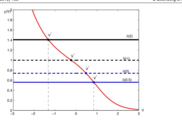
Proof. Using the electroneutrality conditionsα1l1+α2l2 =α1r1+α2r2 =0, equation (3.2)
becomesχ (V )=δ(r1/l1)where
χ (V )= 1−x2+x1e
α2V0+(x
2−x1)eα2V
1−x2+x1eα1V0+(x2−x1)eα1V
and δ(ρ)= e
α2V0−ρ
eα1V0−ρ. (4.2) The left hand side is positive. Thus, a necessary condition for the existence of a real root of (3.2) is(l1eα1V0−r1)(l1eα2V0−r1) >0, or equivalently,
(l1eα1V0−r1)(l2eα2V0−r2) >0. (4.3)
The functionχ (V )is decreasing inV with the range(0,∞). Therefore, the necessary condition (4.3) implies that (3.2) has a unique solution, which leads to a reversal permanent chargeQ∗.
For the statement on the signs ofQ∗andV∗, we demonstrate the proof for (i). Under the conditions in (i), it can be verified directly that
χ (V0)=
1−x2+x1eα2V0+(x2−x1)eα2V0
1−x2+x1eα1V0+(x2−x1)eα1V0
> l1e
α2V0−r 1
l1eα1V0−r1
=δ(r1/l1).
Sinceχ (V )is decreasing inV, we haveV∗ >V0. Now, from (3.5),
Q∗ =α1(l1−J1x1)
eα2(V0−V∗)−eα1(V0−V∗)
.
The right-hand-side is positive due tol1−J1x1 >0 from (3.8),α1 >0> α2 andV∗ >V0.
One concludes thatQ∗>0.
We comment that case (i) and case (iv) are equivalent—one can be obtained from the other by flipping the channel. Similarly, case (ii) and case (iii) are equivalent.
Example 4.2.We provide a simple numerical study to illustrate our result. Considerα1 =2,
α2 = −1,V0 =0.1,l1 =1,l2 =2,r1 =r,r2 =2r,x1 =1/4 andx2 =3/8. Recall, from
(4.2),V =V∗solvesχ (V )=δ(r)where
χ (V )= 5 + 2e
−1/10+ e−V
5 + 2e1/5+ e2V andδ(r)=
e−1/10−r
e1/5−r .
Figure2shows the graph ofχ (V )and the lines ofδ(r)withr=0,0.5,2,∞. Forr=0.5 and 2, the corresponding values are given in table1.
Figure 2.Values ofV∗with differentrin example4.2.
Table 1. Data in the first row correspond to case (i) in proposition4.1and second row to case (iii).
r1=r V∗ Q∗ J1 J2
0.5 0.8482 3.356 0.4475 0.895 2 −1.324 −41.09 −0.829 −1.658
4.1.2. An interesting property of individual ion fluxes. In attempting to understand how the
reversal permanent chargeQ∗affects individual ion fluxesJ1andJ2,an interesting feature was discovered that may not be totally intuitive. Take the case (i) in proposition4.1withα1 =1
andα2 = −1 for example. To make the discussion easy to follow, we useJk(Q2)to denote
the dependence ofJkon the valueQ2for the permanent chargeQin (A3). In this case,l1=l2
andr1=r2. Ifr2 < e−V0l2(and hencer1 < eV0l1as well), thenJ1(Q2) >0 andJ2(Q2) >0
from (1.6). IfQ=0, thenIandV0have the same sign; that is,I=J1(0)−J2(0) >0 since
V0>0. AsQ2increases from 0 toQ∗>0, one might suspect that the ion fluxJ1(Q2)of the
positively charged ions should tend toreducewhile the ion fluxJ2(Q2)shouldincrease, and
the valueQ∗>0 would be the right amount of positive charges to produce zero current. This is NOT true in general. In fact, we have the following result.
Proposition 4.3. Consider n = 2 with α1 = 1 and α2 = −1 (so l1 = l2 = l and
r1 = r2 = r due to electroneutrality boundary conditions). Assume r < e−V0l and
V0 > 0 (so that J1(0) > J2(0) > 0). For some choices of parameters, one may have
J1(0) > J2(0) > J1(Q∗)=J2(Q∗).
Proof.It is known (see, e.g. [1,38]) that, forQ2=0,
J1(0)=(l−r)
1 + V0 lnl−lnr
andJ2(0)=(l−r)
1− V0 lnl−lnr
.
Therefore,J2(0) > J1(Q∗)=J2(Q∗)if and only if
(x2−x1)eV ∗
> le
V0−r
l−r
lnl−lnr
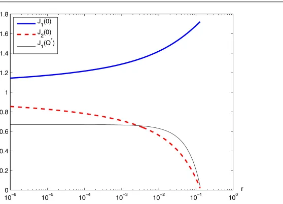
lnl−lnr−V0 −
Figure 3. Graphs ofJ1(0),J2(0)andJ1(Q∗) = J2(Q∗)as functions ofr. The top curve is the graph ofJ1(0), the dashed curve is that ofJ2(0), and the thin curve is that ofJ1(Q∗)=J2(Q∗).
It follows from (3.2) thatV∗satisfies
eV∗ =B+ B
2+ 4(x
2−x1)2(le−V0−r)(leV0−r)
2(x2−x1)(le−V0−r)
,
whereB=((1−x2)l+x1r)(eV0−e−V0). For fixedV0, asl/r→ ∞, one has
eV∗ → (1−x2)(e
2V0−1)+ (1−x
2)2(e2V0−1)2+ 4(x2−x1)2e2V0
2(x2−x1) .
Asl/r→ ∞, the right-hand-side of (4.4) approaches(1−x1)eV0−1 +x 2.
Therefore, for any fixedx1andx2with 0< x1< x2 <1, the inequality (4.4) holds ifV0
is large enough andl/ris large enough.
Example 4.4.In this example we consider
α1=1= −α2; V0=2, l1 =l2=1, r1 =r2=r; x1 =1/4, x2 =7/8
and varyr in [10−6,0.1296] (0.1296 < e−2). The graphs ofJ1(0),J2(0), andJ1(Q∗) = J2(Q∗), which are considered as functions ofr, are plotted in figure3. Forr < 0.0027, one
hasJ2(0) > J1(Q∗)=J2(Q∗).
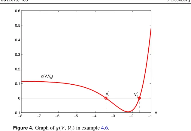
4.2. n=3withα1=1,α2 =2andα3 = −1
This case might be for a mixture of Ca++Cl−
2 and Na+Cl−.
In this case,l1+ 2l2−l3 =0 andr1+ 2r2−r3 =0. We will show it is possible that,
for fixedV0,g(V ,V0)has two real zeros, each leading to a reversal permanent charge—a new feature that does not occur for ion solutions with only two distinct valences.
![Figure 1. [j,−]) on Zj uof �[j,−]in α(N Band, and connects ‘landing’ points of[−1+]in [−1+] and ‘departing’ pointsj �js �j, ω(Nj,) w �[j−1,+]is a singular layer at x = x from to and[−]from toj−1 Bj−1 Zj �j, � Z : A singular orbit over [xj−1, xj] projected to the space of variables,αscj.](https://thumb-us.123doks.com/thumbv2/123dok_us/890557.601543/8.595.156.419.86.260/connects-landing-departing-pointsj-singular-singular-projected-variables.webp)