Munich Personal RePEc Archive
A Refinement of the Relationship
between Economic Growth and Income
Inequality in Developing Countries
Fawaz, Fadi and Rahnamamoghadam, Masha and Valcarcel,
Victor
Jamestown College, Texas Tech University, Texas Tech University
8 April 2014
Online at
https://mpra.ub.uni-muenchen.de/55268/
A Refinement of the Relationship between Economic Growth and
Income Inequality in Developing Countries
THIS DRAFT:
April 8, 2014
Fadi Fawaz
♥; Masha Rahnamamoghadam
♣; Victor Valcarcel
♣1 ♥Department of Economics, Jamestown College, Jamestown, ND 58405 ♣Department of Economics, Texas Tech University, Lubbock, TX 79409
Abstract: There is mixed evidence in the literature of a clear relationship between income inequality and economic growth. Most of that work has focused almost exclusively on developed economies. In what we believe to be a first effort, our emphasis is solely on developing economics, which we classify as high-income and low-high-income developing countries (HIDC and LIDC). We make such distinction on theoretical and empirical grounds. Empirically, the World Bank has classified developing economies in this manner since 1978. The data in our sample is also supportive of such classifications. We provide a theoretical scaffolding that uses asymmetric credit constraints as a premise for separating developing economies in such a way. We find strong evidence of a negative relationship between income inequality and economic growth in LIDC to be in stark contrast with a positive inequality-growth relationship for HIDC. Both correlations are statistically significant across multiple econometric specifications. These results are robust to degree of persistence in the variables of interest as well as a measure threshold of income that is estimated endogenously for our sample.
JEL Classification:E32, O1, O4
Keywords: Income inequality, economic growth, Gini coefficient, credit constraints, collateral
♣
Fadi Fawaz Email: [email protected]
♣
Masha Rahnamamoghadam Email: m.rahnamamoghadam @ttu.edu
♣
1. INTRODUCTION
Elucidating a clear connection between economic growth and income inequality is arguably one
of the most important economic questions of our day. There was much interest in income inequality
in developing countries in the 1960s that diminished as these countries were faced with more pressing
issues including declining growth rates and debt problems (Gillis, 1992). With increasing financial
globalization and recent important sociopolitical developments, the relevance of the question is
experiencing a resurgence that is not likely to diminish in the future. A probable endogeneity in the
relationship, exacerbated by pronounced identification issues and numerous measurement concerns,
raises the difficulty of attaining an incontrovertible answer. Consequently, there is neither a
theoretical consensus, nor consistent empirical evidence that would lead to the conclusion of a strong,
or weak, relationship that is positive or negative.
In seminal work, Kuznets (1955) showed that since the beginning of the 19th century, the process
of economic growth had reduced income inequality in most countries by increasing per capita
income, which came hand-in-hand with labor movements from the agricultural to industrial sectors.
He showed that the process led to a gradual increase in income inequality at the early stages of
development, and as economic growth continued, it gradually led to reductions in income
inequality—the famous Kuznets’ inverted U-shaped curve.
Since Kuznets, an abundance of theoretical models have been advanced. However, many of the
competing theories have offsetting effects leading to an ambiguous net effect of inequality on
economic growth. Empirical lessons are not much better as they tend not to be robust. For example,
Benabou (1996) and Perotti (1996), among others, find increases in inequality tend to be associated
with lower economic growth, whereas Forbes (2000) predicts the opposite.
Many of these competing theories may be classified under three broad categories: i)
socio-political, ii) savings rates and tech spillovers, and iii) credit-market asymmetries— the one this paper
operates in.
Income inequality may have some sociopolitical implications if it serves to incentivize behaviors
that are disruptive to economic activity such as crime, political instability, and revolution—thus, these
might lead income inequality to detract from economic growth. Insofar as political unrest might lead
to revolution, or the toppling of regimes, governments might engage in some redistribution of
resources from the rich to the poor [see Perotti (1993), Alesina and Rodrick (1994), Persson and
Tabellini (1994), among others] in order to mitigate the possibility of regime change. If a greater
degree of inequality leads to greater redistribution for political purposes, and this redistribution
generates more distortions [See Barro (2000) for explanations of tax distortions from financing
supply] it may lead to reductions in economic growth. However, if higher income inequality
incentivized the type of redistribution that served to allocate idle resources from the rich to poorer
(but more productive) agents, then this redistribution could generate a positive relationship between
higher inequality and economic growth.
There is some mixed evidence that low-income individuals tend to have a higher marginal
propensity to consume than high-income individuals. If that is the case, then a redistribution from
high-income to low-income individuals might serve to lower the aggregate saving rate in the
economy. Thus, a rise in income inequality might lead to higher levels of domestic investment that
would foster economic growth. Another avenue for this mechanism is that of technological advances.
If technological improvements serve to reduce setup costs for investment (e.g., reductions in price of
computing reduce barriers to entry in computing-intensive activities) and this leads to higher
investment by lower-income agents (with lower individual saving rates) then this could induce a
positive relationship between higher degrees of income inequality and economic growth.
Finally, in an economy with credit market asymmetries, credit avenues may not be widely open to
both high- and low-income individuals. With limited access to capital markets, the undertaking of
investment opportunities will depend, to some degree, on individual holdings of assets and levels of
income. In an economy where credit is highly constrained to wealthy individuals, a redistribution of
assets and income from the 'idle rich' to the 'productive poor' might raise the average productivity of
investment. In this case a reduction in inequality might foster higher economic growth. On the other
hand, in an economy where productivity gains require high levels of human capital, investment
requires steep setup costs, or firms' profitability is only sustainable beyond a certain size of company,
then—with limited access to capital markets—any of these factors present clear advantages to agents
with high income or a high concentration of assets. In this case higher income inequality might favor
economic growth.
As the next section highlights, much of the empirical literature on the relationship between
income inequality and economic growth focuses either on purely developed economies or on large
panels with a larger share of developed than developing economies. Two important examples are
Barro (2000) and Forbes (2000). In this paper, we focus exclusively on developing economies as
characterized by the World Bank. This encompasses a vast swath of countries (we consider 111).
Thus, we classify these economies as high-income developing countries (HIDCs) and low-income
developing countries (LIDCs)—according to both the World's Bank classification as well as our own
classification based on an income threshold that is endogenously estimated by our model. Because, a
priori, there may be wide differences across the two groups of countries in terms of institutions,
relationship (between income inequality and economic growth) to differ across income groups. The
central thesis of this paper is that firms in HIDC economies may enjoy higher levels of collateral, and
therefore more robust access to capital markets, than companies in LIDC economies, which may be
faced with more constrained access to credit markets.
As a preview of our results, we find that the relationship between inequality and growth seems
significantly positive for HIDC and significantly negative for LIDC. The rest of this paper is
organized as follows: Section 2 provides a brief outline of the empirical findings in the literature.
Section 3 advances a brief theoretical illustration in which the relationship can be sensitive to income
thresholds as functions of the availability of collateral. Section 4 presents various empirical
applications and discusses results. Section 5 concludes.
2. THE EMPIRICAL RELATIONSHIP BETWEEN INEQUALITY AND GROWTH
A clear empirical relationship between income inequality and economic growth remains elusive.
Difficulties stem from: i) the evident endogeneity issue, ii) lack of reliable data, and iii) sensitivity to
different econometric approaches.
Analysis of this kind begs the question of whether economic growth responds to changes in
income inequality or whether income inequality responds to economic growth (in any direction). For
the latter, this suggests placing income inequality as the dependent variable in the regression and
placing some measure of economic activity, or growth, as the explanatory variable on the right-hand
side [see Partridge (1997) and Fawaz et al. (2012) for two such examples of this approach]. However,
the former question—which involves considering economic growth as the dependent variable on the
left-hand side and income inequality as a regressor—is possibly much more popular, and it is the
approach we take here.
Benabou (2000) provides a comprehensive review of studies of this question, most of which
relied on cross-sectional analysis of cross-country data that differed greatly in terms of quality. The
influential work of Deininger and Squire (1996), who compiled a more comprehensive international
dataset on income inequality (the Gini measure), is widely regarded as an important quality
improvement in the data. Their database allows for more straightforward cross-county comparisons in
inequality.
The sign in the relationship between inequality and economic growth seems sensitive to different
econometric methodologies. Various applications of the ordinary least squares (OLS) methodology
typically find a negative relationship between income inequality and growth. For example, Persson
and Tabellini (1994) interpret a higher relative position of the middle quintile of income as a higher
1960-1985 period for a cross-section of countries. Another notable example is Alesina and Rodrick
(1994) who, over the same period, find a negative relationship between Deininger and Squire's Gini
coefficient of inequality and economic growth for a different cross-country sample. Along with
Perotti (1993), these papers find a negative relationship to be motivated by the redistribution
mechanism explained earlier. Galor and Zeira (1993) also find that reducing wealth inequality can
promote economic growth, but the mechanism they employ there is one that advances credit
constraints as the possible explanation.
With the advent of the Gini measure, which enables estimation of more complete or higher
quality panels, other authors relied on a fixed effects (FE) econometric approach, arguing that OLS
estimates may be biased by omitted country-specific effects. In addition, OLS regressions generally
contemplate inequality at long lags by starting at an early date of economic growth, around 1960, and
projecting it onto the next 25 years. FE models typically consider shorter lags of five-year periods.
Generally this econometric approach results in a positive relationship between inequality and
economic growth. Two notable examples are Galor and Tsidon (1997) and Forbes (2000). The former
argue that in the presence of sustained technological improvements high-skilled labor tends to
concentrate in high-tech industries, which may deepen income inequality while fostering economic
growth. The latter controls for time-invariant country-specific effects to reduce a potential source of
omitted variable bias.
Finally, Quah (2001) and Panizza (2002) find little or no stable relationship between inequality
and economic growth. With another methodology based on a three-stage least squares (3SLS)
estimator procedure, Barro (2000) also finds no clear relationship between inequality and growth.
However, by employing the usual sample of rich countries, typically used in other FE models, and
augmenting it with a sizeable number of poorer countries, he finds a different relationship between
the poor countries and the rich countries.
A possible explanation for the ambiguity in the relationship between income inequality and
economic growth and its sensitivity to various econometric techniques is that the relationship could
be nonlinear. For example, estimates in Barro (2000) and Forbes (2000) are consistent with a different
relationship at short horizons than at long ones. Overall, the different results could stem from attempts
to extract different structural explanations from the same reduced form evidence—a point
persuasively made by Banerjee and Duflo (2003).
In this paper we focus on developing economies, where the relevance of the question is likely to
remain high in the coming years. We explore the possibility of nonlinearity in the inequality-growth
relationship in developing economies as a function of income distribution of these countries. Our
in the introduction—namely, credit market asymmetries. Our hypothesis is one of limited
accessibility to credit markets for developing countries below a certain threshold of income. In the
next section, we provide a brief theoretical illustration to motivate subsampling developing
economies into HIDCs and LIDCs and allow the correlation to be different across the two income
groups.
3. COLLATERAL, INCOME INEQUALITY AND ECONOMIC GROWTH IN DEVELOPING ECONOMIES
In the presence of diminishing marginal product of capital, economic growth can be fostered in
economies that enjoy robust markets where the owners of the factors of production and the users of
those factors can meet. For some degree of inequality, private investment can be enhanced when
those agents with a lot of assets (perhaps not fully employed to capacity) can lend them to poorer, but
more productive, agents. Thus, in the face of inequality, robust capital markets facilitate such
transactions, which can be growth-enhancing. Credit constraints present an impediment to this
process and, therefore, can have a deleterious effect on growth.
We present a similar theoretical model to Benabou (1996) and we augment it to consider two
economies—one high-income and one low-income. We begin with two fairly innocuous assumptions:
One, the 'grease' that facilitates credit transactions is the availability of collateral (denoted by
ϕ
).Two, the availability of collateral will be generally higher in higher-income countries than in
lower-income countries (CP).
Take a high-income and a low-income developing economy. The high-income economy is
classified as such because its national income is above some threshold aggregate level of income
( )
Y
. The national income for the low-income economy is below thatY
threshold. Each economy is populated with N-many arbitrary number of firms. Firm j ownsk
0,jinitial units capital at the beginning of period t and produces according to the following technology0 1
j j
y
=
Ak
α <α < (3.1)where
k
jis the amount of capital firm j employs and, because of knowledge spillovers, the factorproductivity
( )
A
for firm j depends on the aggregate level of capital stock that accumulates according to1
t t t t
where
s
andδ
denote the exogenous saving and depreciation rates, respectively, andY
t is the aggregate level of output, or income, in the economy at period t that is derived from aggregating allproduction across the N firms 1
N
t j
j
Y y
=
=
∑
.Let
ϕ
denote the available level of collateral a given firm j might be endowed with. We assume that this collateral is a function of the income that the company generates as followsj
y
ϕ µ
=
(3.3)where
µ
>
0
denotes the share of income the firm desires to hold as collateral to leverage future loans. Thus, collateral is assumed to be a positive and increasing function of income for the firm.However, we do not assume that function to be smooth. In other words, we assume that collateral
tends to dry up quickly for firms that underperform. Thus, we assume
1 0
0 . .
j
if y Y
N o w
ϕ
> ≥=
In the aggregate, our assumption implies that for countries with a large share of the N firms
producing below the average threshold level of income 1
Y N
, it is more likely that the aggregate
level of income is below the threshold. The availability of collateral in such a LIDC may be greatly
reduced. The converse, then, suggests that countries with income above this threshold (HIDCs) may
be endowed with higher levels of collateral and, thus, better access to capital markets.
Thus, an agent can employ more
( )
k
j capital than it owns(
k
0,j)
by borrowing at the beginning of the period but only if it has collateral(
ϕ
>
0)
. In the absence of collateral, the firm can either employ as much capital as it owns(
k
j=
k
0,j)
, or employ less(
k
j<
k
0,j)
and lend the difference to collect a market rate (r>0).Thus, firm j solves the following problem
0,
(
)
j
j j j
k
Max Ak
α−
r k
−
k
−
ϕ
(3.4)by finding an optimal level of capital that maximizes its income net of its cost of borrowing. If
increasing function of factor productivity and capital share of output and a decreasing function of the
cost of borrowing. Thus, yielding the following solution
1 1 *
j
A
k
r
α
α
−
=
(3.5)If the aggregate level of capital is composed of the sum-total of all firms' capital stock
1
N
t j
j
K k
=
=
∑
and each firm concluded(3.5)
was its optimal level of capital and chose to employ thatlevel of capital, it is trivial to show the aggregate level of income for that country would be consistent
with Frankel (1962) standard AK model (where
Y
t=
AK
twith A denoting total factor productivity). Combining this with(3.2)
, it is also quite tractable to conclude that along the balanced growth path,output would grow at the same rate as the aggregate capital stock so that
1
t t
y k
t
K K
g g sA
K
δ
+ −
= ≡ = − (3.6)
Benabou (1996) shows that in the event of no borrowing by any firm in the economy, output would grow at a slower rate than
(3.6)
.On the other hand, if a firm j had collateral
(
ϕ
>
0)
and it were to be more representative of firms in a HIDC where (Y
t>
Y
), then solving the firm's problem(3.4)
along with the definition ofcollateral
(3.3)
would yield the following solution(
)
11**
1
j
r
A
k
r
α
µ α
−
+
=
(3.7)Inspecting
(3.7)
in comparison with(3.5)
—and given that both r>0andµ
>
0
byconstruction— reveals that k**j >k*jthe optimal level of capital in a market with more collateral (less
constrained credit market) is higher than the level of capital in a market with less collateral (more
constrained credit markets). Optimal condition
(3.7)
suggests that the optimal level of capital k**j forfirm j is an increasing function of the desired level of collateral
µ
. Thus, higher levels of collateral(or less constrained credit markets) may lead to faster accumulation of capital and therefore be
conducive to higher economic growth. This suggests that income inequality in HIDC economies with
relationship between income inequality and economic growth in LIDCs, typically with lower levels of
collateral, might go in the other direction.
4. EMPIRICAL APPLICATIONS
We undertake a number of approaches to study whether income inequality promotes (or detracts
from) economic growth for a large panel of developing countries classified as either high-income or
low-income. Our hypothesis is that the impact of income inequality on economic growth is a function
of the availability of collateral—and that, in turn, varies with national income. Thus, we follow the
World Bank (2012) classification of developing countries into LIDCs and HIDCs. However, it could
be argued that this classification—as established by the World Bank—could be considered somewhat
arbitrary.2
We employ annual data from 1960 to 2010 on 111 countries from the World Development
Indicator (WDI) database of the World Bank (2010).
Thus, our final approach is to consider a threshold model and let our sample determine
endogenously whether there is a natural cutoff point in income across these countries to distinguish
between HIDC and LIDC. We conduct our analysis with an FE model, as well as a dynamic panel
approach where we regress our endogenous variable—economic growth—on various measures used
by Barro (2000) and Forbes (2000) encompassing income inequality, industrial prices, and human
capital formation.
3
t
y
The variables we select are commonly used in
empirical studies of inequality and economic growth. These variables are employed by Forbes (2000),
who in turn picks these variables following the work of Perotti (1996), which she characterizes as "his definitive study finding a negative effect of inequality on growth" (p.872). Our dependent variable
( ) is annual percentage change in per capita gross national product (GNP) at constant 2005
purchase power parity (PPP) prices.4 We include the Gini coefficient in our set of regressors as our
measure of income inequality—an updated version of the Deininger and Squire (1996) dataset from
the World Bank (2010).5
2
The World Bank issued the first World Development Report in 1978. Their classification of developing countries has changed over time. For instance, in 1978 they subclassify these countries between "low" and "middle income" countries. The installment we use in this paper (WDR 2012) divides developing countries into "low" and "high" income. The benchmark criteria has also changed. For example, in 1978 the benchmark was based in per capita GNP (US$250) whereas in 2012 the benchmark was based in Gross National Income (US$1,035).
We include net male (Msch) and net female (Fsch) enrollment ratios. These
3
Given that, for many countries, this data set does not contain schooling information before 1970, the closest comparable variable from Barro and Lee (1993) is selected for the period of 1960-1969.
4
An international dollar has the same purchasing power over GNI as a U.S. dollar has in the United States. GNI is the sum of value added by all resident producers plus any product taxes (less subsidies) not included in the valuation of output plus net receipts of primary income (compensation of employees and property income) from abroad.
5
measure the number of students of official school age who are enrolled in primary school as a share
of the total population of children who fall in the corresponding official school age group. We employ
the PPP ratio of investment divided by the exchange rate relative to the United States (PPPI) from the Penn World Tables 6.1. This variable is commonly used in the open economy literature to proxy for
market distortions that affect the cost of investment (see Forbes 2000).
4.1 Benchmark Model
Our sample covers annual data on several macroeconomic aggregates in 55 countries
classified as LIDC according to the World Bank, and 56 countries classified as HIDC from 1960
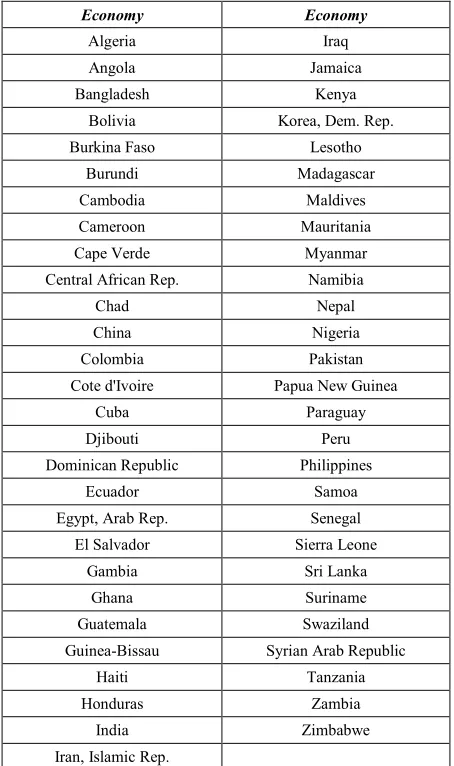
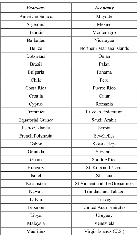
to 2010 (the names of the countries sampled are provided in Tables 1 and 2).
[INSERT TABLES 1 & 2 HERE]
As a first step, we draw inferences on the relationship between income inequality and economic
growth in developing countries by considering a standard model in the literature (see Barro 2000,
Forbes 2000, Caselli et al. 1996, Perotti 1996, among others)
1 1 2 1 3 1 4 1 5 1
it i it it it it it it
y =
α α
+ G − +α
y − +α
Msch − +α
Fsch − +α
PPPI − +ε
(4.1)it i it
ε
= +
υ µ
(4.2)0 6
i
Z
iα α α
=
+
(4.3)These are one-way error component regression models for our two categories of developing
countries, LIDC and HIDC, where our dependent variable yitis per capita GNP growth for country i at time t. Git-1is the income inequality coefficient (Gini) for country i at time t-1.
Mschit-1 and Fschit-1 are male and female school enrollments, respectively, all drawn from the World's Bank WDI database. We also follow Forbes (2000) in including the price level of
investment for country i at time tPPPIit-1 as a proxy for market distortions. In performing this type of analysis, one concern is the possibility of feedback from income inequality to growth if
the regression is performed contemporaneously. Using lagged income inequality on the
right-hand side might ameliorate the endogeneity issue (see Temple 1999). It also allows us to assess
the dynamic effects of income inequality on growth.
In the one-way error model of (4.2), υidenotes the time-invariant and unobservable
country-specific effects and μit denotes the remaining unexplained disturbance with mean zero
and variance-covariance 2
nt
I
ν
σ . Ζi in (4.3) represents unobserved characteristics of the shifter
[INSERT TABLE 3 HERE]
Table 3 summarizes the regression results outlined by the system (4.1)-(4.3). Of foremost
importance is the statistically significant estimates of the inequality coefficient. This table shows
evidence that the relationship between income inequality and economic growth is in stark contrast
between LIDCs and HIDCs. Increases in inequality seem to be positively related with economic
growth in HIDCs. This result seems consistent with our theoretical framework if firms in HIDCs
have generally higher levels of collateral or easier access to credit markets. Conversely, higher
levels of income inequality seem detrimental to economic growth in LIDCs. This result is, at least
in principle, consistent with the findings in Barro (2000) of a negative correlation between
income inequality and economic growth in "poorer" countries.
It can also be explained in the context of our theoretical hypothesis in Section 3. If LIDC
economies are populated with firms that do not enjoy any meaningful levels of collateral, then
they might be faced with little access to capital markets, which would have a deleterious effect on
capital accumulation, and hence, economic growth.
4.2 A Dynamic Model to Control for Persistence
Ignoring the importance of lagged dependent variables, when they are persistent, could
lead to an omitted variable bias problem. Thus, we model a variant of (4.1)-(4.3) with all
variables entering the model in first differences and where we regress our endogenous, economic
growthyitq, variable in a dynamic setting as follows:
(
1) (
1 2)
(
1) (
1)
q q q q
it it it it it it it it
y −y − =
β
y − − y − +λ
Χ − Χ − +ε
−ε
−(4.4)
where
q
∈
[
HIDC LIDC
,
]
according to the World Bank Classification that was also employed in the previous section. The matrix of regressors Χcontains the gini(
G
it)
coefficient of incomeinequality,MschitandFschitas measures of male and female school enrollments, respectively, and the
price level(PPPIit)of investment.
If there was substantial correlation present between the lagged dependent variables, the OLS
estimator would be severely biased (Hsiao 2003) and exacerbated as the variance of the
individual effects increases. Anderson and Hsiao (1981) describe an instrumental variable
implementation that, in our context, involves choosing either yitq−2or
(
yitq−2− yitq−3)
as anlags) are not the only two viable instruments. For our purposes any lag, beyond the second, may
be uncorrelated with the error term while not necessarily uncorrelated with the lagged
endogenous term. Arellano and Bond developed a procedure that treat the model as a system of
equations, one for each period, where the matrix of differenced instruments is built recursively
and estimated within a generalized method of moments (GMM) approach.6
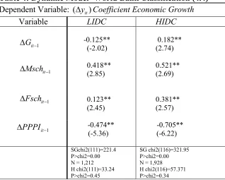
[INSERT TABLE 4 HERE]
Table 4 shows results of the (4.4) regression applied to two panels: one panel of 56
countries classified as HIDCs by the World Bank, and a second panel of 55 countries classified as
LIDC by the World Bank. Here again, the income inequality coefficient is negative for LIDC
economies and positive for HIDC economies. Both estimates are statistically significant. Thus,
the stark contrast, across income groups, in the relationship between income inequality and
economic growth seems robust to the degree of persistence in the variables of interest.
Furthermore, all models thus far show that male and female school enrollments are significantly
positively related to economic growth.7 Finally, market distortions, as proxied by the price of
investment, are negatively correlated with economic growth across all specifications. This result
is consistent with findings in Perotti (1996), Forbes (2000), and others.
4.3 An Endogenous Threshold Model
All results described thus far are based on the World Bank (2012) classification (outlined
in Tables 1 and 2) of developing countries into 55 that fall in the category of LIDCs, and 56
countries classified as HIDCs. However, it could be argued that this classification may be
somewhat arbitrary. For robustness, we consider a generalized threshold approach where we let
the model find the measure of income that best fits the data. To that end we specify the following
model of economic growth
(
y
it)
for country i at period t that combines both types of countryclassification:
( ) ( )
HIDC LIDC
it it it it
y = y I inc>Y + y I inc<Y +
υ
(4.5)
6
With this differenced-GMM approach the endogenous variable is properly instrumented with suitable lags of its own levels—other exogenous regressors and outside variables may enter the matrix of instrument in a standard way. However, with this differenced-GMM Arellano-Bond estimator, the lag levels may be poor instruments for first differences in models (like ours) in which highly persistent variables are considered. Thus, we opt to make use of an augmented version—a system-GMM approach—first described in Arellano and Bover (1995). For details on this estimation procedure, see Blundell and Bond (1998). We applied the XTABOND2 procedure in STATA, which conducts a finite-sample correction to the two-step covariance matrix to correct for the downward bias of the standard errors (Windmeijer 2005).
7
Where Yis some income cutoff point for which the country is classified as a LIDC or a
HIDC based on a generalized threshold approach following Hansen’s (1996, 2000) threshold
procedure. This method searches over values of the threshold using conditional OLS regression
based on a sequential search over all possibleY.8
We then subdivide the sample and test for additional threshold levels. For the subsamples
of observations that exceed the threshold level, the Lagrange multiplier (LM) statistic was too
small compared with the critical value. We conclude that no additional threshold levels are
present. Our results on the economic growth relationship with income inequality seem supportive
of the World's Bank notion that classifying developing countries as high income versus
low-income is warranted. According to results from equation (4.5), the estimated cutoff point for per
capita income suggested by the data is $1,348. Our estimated threshold suggests a
re-classification from the World Bank's in Table 2 in which four countries (Algeria, Colombia,
Dominican Republic, and Paraguay) that were classified as LIDC according to World Bank are
classified as HIDC according to our implied threshold. We re-estimate the dynamic panel model
of (4.4) under this new classification.
[INSERT TABLE 5 HERE]
All results of the dynamic panel approach under the estimated income threshold are
qualitatively consistent with those of the dynamic panel under the World Bank classification. For
robustness, we re-estimate the benchmark model of (4.1)-(4.3) with the income threshold, we
endogenously estimated, as an alternative to taking the World Bank's threshold as given.
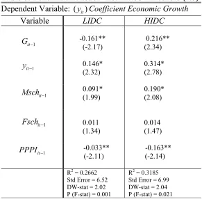
[INSERT TABLE 6 HERE]
Qualitatively we get the same results in our benchmark model, whether we employ the
threshold corresponding to the World Bank classification, or the one that our data set suggests.
Overall, the results look robust to whether we employ the threshold employed by the
World Banks or our own in all specifications we employ. The qualitative robustness of our results
based on our endogenously estimated threshold suggests that the benchmark established by the
World Bank seems a fair representation of developing economies, and one that would seem
consistent with what the data suggests.
8
5. CONCLUSION
Over the years there has been a plethora of studies that attempt to find an unequivocal picture on
the question of whether income inequality is detrimental to long-term economic activity or whether it
can enhance economic growth. A clear answer has remained elusive. A qualitative prediction seems
sensitive to measurement and methodological choice. Much of the previous work on this topic was
hampered by little availability of cross-country measures of inequality. This problem was especially
salient in developing economies. Many empirical attacks that relied on OLS estimations of
cross-sections of developed economies have predicted a negative effect of income inequality on economic
growth. Arguing that OLS may lead to biased results, the next step was to consider FE models with
limited dynamics (5-year periods). This approach typically found a positive relationship between the
inequality of developed economies and their economic growth.
In an influential paper, Barro (2000) finds no relationship between those variables in developed
economies. So the literature has spanned the full set of possible predictions: positive, negative, or no
relationship between income inequality and economic growth. However, by combining developed and
developing economies, Barro finds a stark contrast on the inequality-growth question. Our own
results would seem consistent, at least in principle, with those. An important distinction in our
contribution is that we focus exclusively on developing economies. These economies have routinely
been ignored in the literature, but we argue that their importance to the world economy is not likely to
dwindle (just the opposite) and, thus, the relevance of our question of inequality-growth in these
countries is not likely to diminish either.
The lack of consensus in the literature on a clear relationship between income inequality and
economic growth could be an unintended consequence of imposing a basic linear structure (OLS, FE)
on what could be a nonlinear relationship. So different predictions could arise from lending different
structural interpretations to the same reduced-form evidence (Banerjee and Duflo 2003). We present
in Section 3 a simple theoretical model that advances a relationship between income inequality and
economic growth that is far from linear. That nonlinearity arises from credit market asymmetries
among countries at different levels of income with ensuing differences in available collateral and
access to credit markets. The data strongly supports the notion of building a case for nonlinearity.
We regress economic growth on the Gini measure of income inequality in a panel of 55 LIDCs
classified as such by the World Bank. Then, we conduct the same regression on a panel of 56
countries classified as HIDCs by the World Bank. Following Perotti (1996), Forbes (2000), and
price of investment goods as explanatory variables in these regressions. Human capital measures have
long been considered important explanatory variables in economic growth regressions. See Forbes
(2000) for a comprehensive explanation for the inclusion of market distortion measures in these types
of growth regressions. For our own context, market distortions on the price of investment goods could
have distortionary effects on the valuation of collateral, which is the pillar with which we promote our
nonlinear threshold approach in our theoretical framework.
We find a positive relationship between income inequality and economic growth in HIDCs,
which is in stark contrast with the negative relationship for LIDCs. We estimate an income threshold
endogenously and re-estimate both regressions according to our own threshold. Importantly, the
contrasting qualitative difference (between LIDC and HIDC) in the relationship between income
inequality and economic growth is robust whether we follow the World Bank's classification of
developing economies or whether we classify them accordingly to what the data in our sample
suggests.
It could be argued that these results might be sensitive to the degree of persistence in the variables
included in the regressions. Thus, we estimate variants of the benchmark regression with an
Arellano-Bond specification based on a GMM estimation of a recursive differencing approach. Qualitatively,
all our results are robust to these alternative econometric techniques.
Thus, our results are not sensitive to alternative threshold measurements or econometric
specifications. Such robustness argues for the possibility that the relationship between income
inequality and economic growth is likely nonlinear. The avenue for nonlinearity we advance in this
paper is a nonlinearity in the credit channel vis-a-vis national income. But other nonlinearities could
prove to be just as important. For example, the correlation between income inequality and economic
growth could be time variant even for specific cases of a single country. Another possibility is that the
relationship could be asymmetric. For example, it could be the case that only reductions (but not
increases) in inequality matter for economic growth—or vice versa. These are outside the scope of the
REFERENCES
Alesina, A. and Rodrick, D. 1994, “Distributive Politics and Economic Growth”, Quarterly Journal of Economics,109(2), pp. 465-90.
Anderson, T.W. and Hsiao, C. 1981, “Estimation of Dynamic Models with Error Components”, Journal of the American Statistical Association, 76, pp. 595-606.
Arellano, M., and Bond, S. 1991, “Some Tests of Specification for Panel Data: Monte Carlo Evidence and an Application to Employment Equations”, Review of Economic Studies, 58, pp. 277-297.
_________., and Bover, O. 1995, “Another Look at the Instrumental Variable Estimation of Error-Components Model”, Journal of Econometrics, 68, pp. 29-51.
Banerjee, A., and Duflo, E. 2003, “Inequality and Growth: What can the data say?” Journal of Economic Growth 8 (3), pp. 267-299.
Barro, R. (2000), “Inequality and Growth in a Panel of Countries”, Journal of Economic Growth, 5, pp. 5-32.
Barro, R. and Lee, J (1993), “International Comparisons of Educational Attainment”, Journal of Monetary Economics, 32(3), pp. 363-94.
Benabou, R. (1996), “Inequality and Growth”, in B. S. Bernanke and J. Rotemberg (Eds.), NBER
Macroeconomics Annual, Cambridge, MIT Press.
Benabou, R. (2000), “Unequal Societies: Income Distribution and the Social Contract”, American Economic Review, 90(1), pp. 96-129.
Blundell, R. and Bond, S. 1998, “Initial Conditions and Moment Restrictions in Dynamic Panel Models”,
Journal of Econometrics, 87, pp. 115-143.
Caselli, F.; Esquivel, G.; Lefort, F. 1996 "Reopening the Convergence Debate: A New Look at Cross-Country Growth Empirics" Journal of Economic Growth 1, pp. 363-389
Deininger, K. and Squire, L. 1996, “A New Data Set Measuring Income Inequality”, World Bank Economic Review, 10, pp. 565-91.
Fawaz, F.; Rahnamammoghadam, M.; Valcarcel, V. 2012, “Fluctuations, Uncertainty and Income Inequality in Developing Countries”, Eastern Economic Journal, 38(4), pp. 495-511.
Forbes, K. 2000, “A Reassessment of the Relationship between Inequality and Growth”, American Economic Review,90(4), pp. 869–88.
Frankle, M. 1962, “The Production Function in Allocation of Growth: A Synthesis”, American Economic Review,52, pp. 995–1022.
Galor, O. and Zeira, J. 1993, “Income Distribution and Macroeconomics”, Review of Macroeconomic Studies,60, pp.35-52.
Gillis, M. 1992, “Economics of Development”, New York: W.WNorton & Company.
Hansen, B. 1996, “Inference when a nuisance parameter is not identified under the null hypothesis”,
Econometrica, 64, pp 413-430.
________. 2000, “Sample splitting and threshold estimation”, Econometrica, 68, pp 575-604.
Heston A., Summers A., Aten, B. 2002 Penn World Table Version 6.1, Center for International Comparisons of Production, Income and Prices at the University of Pennsylvania
Hsiao, C. 2003, “Analysis of Panel Data,” Cambridge University Press.
Kuznets, S. 1955, “Economic Growth and Income Inequality”, American Economic Review, 45(1), pp. 1-28.
Panizza, U. 2002, “Income Inequality and Economic Growth: Evidence from American Data”, Journal of Economic Growth, 7(1), pp. 25-41
Partridge, M. 1997, “Is Inequality Harmful for Growth? Comment”, American Economic Review, 87(5), pp. 1019-32.
Perotti, R. 1993, “Political Equilibrium, Income Distribution, and Growth”, Review of Economic Studies
60(4), pp. 755-776.
Perotti, R. 1996, “Growth, Income Distribution, and Democracy: What the Data Say”, Journal of Economic Growth 1(2), pp. 149-187.
Persson, T. and Tabellini, G. 1994, “Is Inequality Harmful for Growth? Theory and Evidence”, American Economic Review, 48(3), pp. 600-621.
Quah, D. 2001,”Some Simple Arithmetic on How Income Inequality and Economic Growth Matter”, LSE Economics Working Paper.
Temple, J. 1999, “The New Growth Evidence”, Journal of Economic Literature, 37, pp.12-156
Windmeijer, F. 2005, “A Finite Sample Correction for the Variance of Linear Efficient Two-Step GMM Estimators” Journal of Econometrics, 26(1), pp. 25-51.
World Development Indicators (WDI) Database 2010, World Bank, Washington, D.C.
World Development Report (WDR) Database 2012, World Bank, Washington, D.C
Error! Main Document Only.Error! Main Document Only.Error! Main Document Only.
Table 1: Low Income Developing Countries (LIDCs)
per capita GNI
≤
US($) 1,035
Economy Economy
Algeria Iraq Angola Jamaica Bangladesh Kenya
Bolivia Korea, Dem. Rep. Burkina Faso Lesotho
Burundi Madagascar Cambodia Maldives Cameroon Mauritania Cape Verde Myanmar Central African Rep. Namibia
Chad Nepal
China Nigeria Colombia Pakistan Cote d'Ivoire Papua New Guinea
Cuba Paraguay Djibouti Peru Dominican Republic Philippines
Ecuador Samoa Egypt, Arab Rep. Senegal
El Salvador Sierra Leone Gambia Sri Lanka
Ghana Suriname Guatemala Swaziland Guinea-Bissau Syrian Arab Republic
Haiti Tanzania Honduras Zambia
Table 2: High Income Developing Countries (HIDCs)
per capita GNI > US($) 1,035
Economy Economy
American Samoa Mayotte Argentina Mexico Bahrain Montenegro Barbados Nicaragua
Belize Northern Mariana Islands Botswana Oman
Brazil Palau Bulgaria Panama
Chile Peru
Costa Rica Puerto Rico Croatia Qatar Cyprus Romania Dominica Russian Federation Equatorial Guinea Saudi Arabia
Faeroe Islands Serbia French Polynesia Seychelles
Gabon Slovak Rep. Granada Slovenia
Guam South Africa Hungary St. Kitts and Nevis
Israel St Lucia
Kazahstan St Vincent and the Grenadines Kuwait Trinidad and Tobago
Latvia Turkey Lebanon United Arab Emirates
Table 3: Benchmark Model -World Bank Classification (4.1)-(4.3)
Dependent Variable: (
y
it)
Coefficient Economic Growth
Variable
LIDC
HIDC
1
it
G
− -0.066**(-2.02)
0.225** (2.14)
1
it
y
− 0.212*(2.19)
0.252* (2.92)
1
it
Msch − 0.080**
(2.14)
0.108** (2.07)
1
it
Fsch − 0.008 (1.24)
0.013 (1.61)
1
it
PPPI − -0.034**
(-2.05)
-0.089** (-2.16)
R2 = 0.2346 Std Error = 7.55 DW-stat = 2.05 P (F-stat) = 0.017
R2 = 0.2986 Std Error = 7.22 DW-stat = 2.06 P (F-stat) = 0.020
T-values in parentheses. **indicates significance at 1%, *indicates significance at 5%
Table 4: Dynamic Model -World Bank Classification (4.4)
Dependent Variable: (
∆
y
it)
Coefficient Economic Growth
Variable
LIDC
HIDC
1
it
G
−∆
-0.125** (-2.02) 0.182** (2.74) 1 it Msch − ∆ 0.418** (2.85) 0.521** (2.69) 1 it Fsch− ∆ 0.123** (2.45) 0.381** (2.57) 1 it PPPI −∆ -0.474** (-5.36)
-0.705** (-6.22)
SGchi2(111)=221.4 P>chi2=0.00 N = 1,212 H chi2(111)=33.24 P>chi2=0.45
SG chi2(116)=321.95 P>chi2=0.00 N = 1,928 H chi2(116)=57.371 P>chi2=0.34
[image:21.612.159.477.429.684.2]Table 5: Dynamic Model -Threshold-Implied
Classification (4.4)-(4.5)
Dependent Variable: (
∆
y
it)
Coefficient Economic Growth
Variable
LIDC
HIDC
1
it
G
−∆
-0.109** (-1.82) 0.182* (2.74) 1 it Msch − ∆ 0.455* (1.81) 0.521** (2.69) 1 it Fsch− ∆ 0.523* (1.83) 0.381** (2.57) 1 it PPPI −∆ -0.203* (-2.56)
-0.705* (-2.57)
SGchi2(102)=393.53 P>chi2=0.00 N = 978
H chi2(102)=55.24 P>chi2=0.54
SG chi2(118))=437.63 P>chi2=0.00 N = 2,162 H chi2(118)=68.80 P>chi2=0.49
Notes: Same as above
Table 6: Benchmark Model - Estimated Threshold (4.5)
Dependent Variable: (
y
it)
Coefficient Economic Growth
Variable
LIDC
HIDC
1
it
G
− -0.161**(-2.17)
0.216** (2.34)
1
it
y
− 0.146*(2.32)
0.314* (2.78)
1
it
Msch − 0.091*
(1.99)
0.190* (2.08)
1
it
Fsch − 0.011 (1.34)
0.014 (1.47)
1
it
PPPI − -0.033**
(-2.11)
-0.163** (-2.14)
R2 = 0.2662 Std Error = 6.52 DW-stat = 2.02 P (F-stat) = 0.001
R2 = 0.3185 Std Error = 6.99 DW-stat = 2.04 P (F-stat) = 0.021
[image:22.612.156.447.412.698.2]