Economic Growth and Health Indicator in Thailand

(1)

Munich Personal RePEc Archive

Does an improvement in health

encourage economic growth?:Case of

Thailand

durongkaveroj, wannaphong

Chiang Mai University

6 February 2014

Online at

https://mpra.ub.uni-muenchen.de/53494/

(2)

" Economic Growth and Health Indicator in Thailand between 1980 - 2011"

Wannaphong Durongkaveroj

*

Abstract

This study aimed at estimating the relationship between economic growth measured by per capita

Gross National Income (GNI) and health indicators including life expectancy and mortality rate under 5 in

Thailand between 1980 - 2011 using Cochrane - Orcutt Model.

The results from revealed that only mortality rate under 5 has a strong relationship with an

economic growth. Thus, the reform in medical and sanitation system in Thailand will be able to stimulate

the economic prosperity and lead to development further.

*

(3)

Introduction

As mentioned by Todaro & Smith (2008), health and education are the main component of human

capital which encourage an economic development. Health and education link each other. Healthy labor

can work with maximum productivity while educated people are easier in learning new technology or

innovation correspondent to skilled labor. Additionally, Besley & Burgess (2003) explained that an

increase in human capital is the core of development. Thus, this study was inspired so as to study that how

can an improvement in health system affect national prosperity. The result of this study will be beneficial

in issuing national policy.

Research Question

Does an improvement in medical and sanitation system can raise citizen's living standard ?

Purpose

To estimate the relationship between economic growth and health indicator in Thailand

Model Specification :

Simple Regression was implemented. There were two models. For the first model, dependent

variable was economic growth and independent variable was life expectancy. For the second model,

dependent variable was economic growth while independent variable was mortality rate under 5. The data

of all three variable was derived from World Bank data base. All data are time series data whose range is

in between 1980 to 2011.

Results

Time Series data, typically, is necessary to test stationarity (Unit Root Test) before taking them to

regression model. Stationary condition displays an acceptable level of data fluctuation. Non - stationary

data is able to lead to the problem of statistical inference or spurious regression. For Unit Root test,

implemented Augmented - Dickey Fuller, per capita GNI is stationary at 10% alpha. Mortality rate under

5 is stationary at 5% alpha and life expectancy is stationary at 1% alpha.

After stationary process, the next step is to find the relationship between dependent and

independent variable through log-linear model. The reason why I use log-linear model because the

(4)

For the first model, per capita GNI and life expectancy. The result was shown in table 1.

[image:4.595.105.465.182.289.2]

Table 1: The relationship between per capita GNI and life expectancy

.

Source:

Author's calculation

According to table 1, there is a statistically relationship between economic growth measured by

per capita GNI and life expectancy. If life expectancy increase by 1 percent, per capita GNI will increase

by 18.05%. R-squared is 78.04 representing strong relationship. However, to use time series data is

required to test Heteroskedasticity and Autoregression.

The result from Heteroskedasticity test was shown in table 2

Table 2: Heteroskedasticity of model 1

Source:

Author's calculation

The result suggests that there is no the problem of heteroskedasticity.

The next step is to test autocorrelation. I used two methods to test including White Test and

Durbin Watson Test (D.W.). The result from D.W. is shown in table 3

Table 3: White Test of Model 1

Source:

Author's calculation

_c ons - 68. 98777 7. 474373 - 9. 23 0. 000 - 84. 25248 - 53. 72307 l ogl i f eex 18. 05407 1. 748746 10. 32 0. 000 14. 48266 21. 62549 l oggni Coef . St d. Er r . t P>| t | [ 95% Conf . I nt er v al ] Tot al 12. 4447875 31 . 401444757 Root MSE = . 30185 Adj R- s quar ed = 0. 7730 Res i dual 2. 73341172 30 . 091113724 R- s quar ed = 0. 7804 Model 9. 71137575 1 9. 71137575 Pr ob > F = 0. 0000 F( 1, 30) = 106. 59 Sour c e SS df MS Number of obs = 32

Pr ob > c hi 2 = 0. 5733 c hi 2( 1) = 0. 32

Var i abl es : f i t t ed v al ues of l oggni Ho: Cons t ant v ar i anc e

Br eus c h- Pagan / Cook - Wei s ber g t es t f or het er os k edas t i c i t y

.

Pr ob > c hi 2( 14) = 0. 0000

Por t mant eau ( Q) s t at i s t i c = 111. 6754

Por t mant eau t es t f or whi t e noi s e

(5)

According to table 3, there is autocorrelation because p - value is able to reject null hypothesis (

Null hypothesis = No autocorrelation). To make sure about this result, I add the lag in to white test. The

result was shown in table 4.

Table 4: White Test (lags 10) of model 1

Source:

Author's calculation

The result still suggested that there is autocorrelation in this model. Then, I test further using

D.W. test ( D.W. value has to be around 2 to reject autocorrelation). The result was shown in table 5.

Table 5: Durbin Watson Test of model 1

Source:

Author's calculation

According to table 5, there is autocorrelation. Then, I also tested further by using Breusch -

Godfrey. It was shown in table 6.

Table 6: Breusch - Godfrey of model 1.

Source:

Author's calculation

From the result of table 6, it is concluded that there is autocorrelation in the model. When

autocorrelation occurred, the result from table 1 (simple regression) cannot use. For correcting, I use

Cochrane - Orcutt Regression. The result was shown in table 7.

Pr ob > c hi 2( 10) = 0. 0000

Por t mant eau ( Q) s t at i s t i c = 110. 2379

Por t mant eau t es t f or whi t e noi s e

. wnt es t q l oggni , l ags ( 10)

Dur bi n- Wat s on d- s t at i s t i c ( 2, 32) = . 096959 . dws t at

H0: no s er i al c or r el at i on

1 27. 025 1 0. 0000 l ags (p) c hi 2 df Pr ob > c hi 2 Br eus c h- Godf r ey LM t es t f or aut oc or r el at i on

. es t at bgodf r ey

(6)

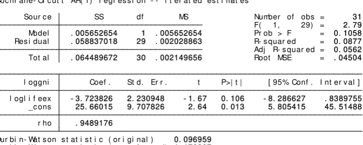
Table 7: Cochrane - Orcutt of Model 1

Source:

Author's calculation

From table 7, the result suggests that Beta (coefficient of independent variable) is indifferent with

zero). It can be implied that life expectancy is not statistically related with per capita GNI.

For the second model, economic growth measured by per capita GNI and mortality rate under 5.

[image:6.595.104.466.127.272.2]

The result from simple regression model was shown in table 8.

Table 8: Regression model of per capita GNI and mortality rate under 5.

Source:

Author's calculation

The results suggest that there is a statistically relationship between per capita GNI and mortality

rate under 5. If mortality rate under 5 is decreased by 1 %, per capita GNI will be increased by 1.17%.

However, due to time series data, the importance of heteroskedasticity and autocorrelation was

realized. The result from heteroskedasticty test was shown in table 9.

Dur bi n- Wat s on s t at i s t i c ( t r ans f or med) 1. 176267

Dur bi n- Wat s on s t at i s t i c ( or i gi nal ) 0. 096959

r ho . 9489176

_c ons 25. 66015 9. 707826 2. 64 0. 013 5. 805415 45. 51488 l ogl i f eex - 3. 723826 2. 230948 - 1. 67 0. 106 - 8. 286627 . 8389755 l oggni Coef . St d. Er r . t P>| t | [ 95% Conf . I nt er v al ] Tot al . 064489672 30 . 002149656 Root MSE = . 04504 Adj R- s quar ed = 0. 0562 Res i dual . 058837018 29 . 002028863 R- s quar ed = 0. 0877 Model . 005652654 1 . 005652654 Pr ob > F = 0. 1058 F( 1, 29) = 2. 79 Sour c e SS df MS Number of obs = 31 Coc hr ane- Or c ut t AR( 1) r egr es s i on - - i t er at ed es t i mat es

(7)

Table 9: Heteroskedasticity of model 2

Source:

Author's calculation

The result from Breusch - Pagan suggested that there was no heteroskedasticity. Then, I tested

further on autocorrelation. Durbin Watson test was shown in table 10:

Table 10: Autocorrelation with Durbin Watson Test of model 2

Source:

Author's calculation

According to table 10, there is a problem of autocorrelation. Then, it was tested further with

Breusch - Godfrey. The result was shown in table 11.

Table 11: Breusch - Godfrey

Source:

Author's calculation

According to the table 11, there is autocorrelation. Additionally, White Test was implemented.

The result was shown in table 12:

Pr ob > c hi 2 = 0. 6845

c hi 2( 1) = 0. 17

Var i abl es : f i t t ed v al ues of l oggni

Ho: Cons t ant v ar i anc e

Br eus c h- Pagan / Cook - Wei s ber g t es t f or het er os k edas t i c i t y

Dur bi n- Wat s on d- s t at i s t i c ( 2, 32) = . 2362855

. dws t at

.

1 22. 913 1 0. 0000 l ags (p) c hi 2 df Pr ob > c hi 2 Br eus c h- Godf r ey LM t es t f or aut oc or r el at i on

. es t at bgodf r ey

(8)

Table 12: White Test of model 2

Source:

Author's calculation

According to table 12, the result confirmed that there is autocorrelation correspondent with

Durbin Watson Test. Then, it is necessary to correct this problem by using Cochrane - Orcutt Ar(1)

[image:8.595.101.284.112.236.2]

Regression. The result was shown in table 13.

Table 13: Cochrane - Orcutt Regression of Model 2

Source:

Author's calculation

According to table 13, it suggested that per capita GNI is statistically related to mortality rate

under 5. If mortality rate under 5 is decreased by 1%, per capita GNI will be increased by 1.086%.

R-squared of 84.54% confirmed that a strong relationship.

Conclusion and Suggestion

As mortality rate under 5 has statistical relationship with economic growth measured by per

capita Gross National Income. It was implied that a decrease of child mortality can help creating a

national prosperity. When child can survive and grow up to be labor, their participation in economic

Pr ob > c hi 2( 10) = 0. 0000 Por t mant eau ( Q) s t at i s t i c = 124. 3094 Por t mant eau t es t f or whi t e noi s e . wnt es t q l ogmor 5, l ag( 10)

Pr ob > c hi 2( 14) = 0. 0000 Por t mant eau ( Q) s t at i s t i c = 127. 1024 Por t mant eau t es t f or whi t e noi s e . wnt es t q l ogmor 5

Dur bi n- Wat s on s t at i s t i c ( t r ans f or med) 1. 227162 Dur bi n- Wat s on s t at i s t i c ( or i gi nal ) 0. 236286

r ho . 836581

(9)

activity, in production sector, service sector, or administration sector can encourage growth. A decrease in

mortality rate can be reduced by a development, improvement, or reform in medical and sanitation system.

Medical equipment and innovation should be supplied and distributed to rural hospital throughout the

country. Doctor, nurse, and hospital worker have to work at their best for utilizing productivity aimed at