Munich Personal RePEc Archive
Estimating Dynamic Demand for Airlines
Diego, Escobari
The University of Texas - Pan American
18 April 2014
Online at
https://mpra.ub.uni-muenchen.de/55408/
Estimating Dynamic Demand for Airlines
∗(Economics Letters, Forthcoming)
Diego Escobari†
April 18, 2014
Abstract
This paper uses an original panel dataset with posted prices and sales to estimate a dynamic demand. We find that consumers become more price sensitive as time to departure nears which is consistent with having lower valuations. This result provides empirical support to a key theoretical implication in Deneckere and Peck [Deneckere, R., Peck, J., 2012. Dynamic competition with random demand and costless search: A theory of price posting. Econometrica 80, 1185-1247] — high-valuation consumers purchase earlier. We also find that the number of active consumers increases closer to departure.
Keywords: Dynamic demand, Consumers’ valuations, Advance purchases, Airlines
JEL Classifications: C23, L93, R41
∗I thank Paan Jindapon and an anonymous referee for helpful comments. Stephanie C. Reynolds provided
outstanding assistance with the data.
†Department of Economics & Finance, The University of Texas - Pan American, Edinburg,
1
Introduction
The demand for airline tickets is dynamic because tickets are offered in advance and
con-sumers can delay their decision to purchase. Beliefs about future prices and sales are
important as multiple sales periods give consumers intertemporal substitution possibilities
and give firms intertemporal arbitrage opportunities (see Deneckere and Peck (2012)). Key
features in the market for airline tickets make the problem interesting. On the demand side
consumers have unit demands, can optimize the timing of their purchase (with potential
delaying costs), and may be uncertain about their travel plans. On the supply side sellers
post prices under aggregate demand uncertainty, capacity is costly and needs to be set in
advance, and unsold seats expire after departure.
In this paper we use an original dataset to estimate a dynamic demand and analyze
how valuations change as the departure date nears. This is an important question because
existing theoretical literature assumes either that valuations are constant across periods
(e.g., Gale and Holmes (1993), Gallego and van Ryzin (1994)), finds that they are increasing
over time (e.g., Dana (1998)), or finds that high-valuation consumers purchase earlier.1
Dana (1998) explains that lower-valuation consumers have incentives to buy in advance
because the presence of high-valuation types (with more uncertain demands) increase the
price they expect to pay in the spot market. Deneckere and Peck (2012) explain that
high-valuation consumers purchase early and low-high-valuation consumers postpone their purchase
decisions to exploit the option to refuse to buy in the future if the sale price exceed their
valuation.
We find strong empirical support that consumers’ purchasing behavior changes as the
departure date nears. When consumers are viewed as making instantaneous decisions we
find that valuations decrease as departure date nears. A dynamic demand interpretation
of our estimates is consistent with the implication in Deneckere and Peck (2012) that
high-valuation consumers purchase earlier. Our dynamic panel estimates are consistent with
agents behaving dynamically and are robust to different assumptions on the endogeneity
of prices and the selection of the instrument list. We also find that the number of active
1
consumers increases closer to departure.
2
Related Literature
Our findings are important to other industries in which consumers face intertemporal
sub-stitution possibilities, for example, during advance sales for hotel rooms, car rentals, and
entertainment and sporting events. Studying demand dynamics is also important in
mod-els for storable goods (e.g., Nevo and Hendel (2013)), durable goods (e.g., Chevalier and
Kashyap (2011)), new products (e.g., Stokey (1979)), habit persistence (e.g., Baltagi and
Levin (1986)), and when sales are concentrated during particular season, e.g. fashion
ap-parel or the Christmas season. Consistent with our results, Bitran and Mondschein (1997)
argues that early buyers of fashion goods are willing to pay more. Two additional related
studies on demand estimation includes Vulcano et al. (2010) who estimate a discrete choice
model with Poisson arrivals for airline revenue management, and DHaultfœuille et al. (2013)
who focus on the French railroad industry to estimate a structural model of demand in the
presence of revenue management.
There is a large empirical literature on airlines that uses fares collected from websites
with nearly all of the work focused on explaining pricing decisions. McAfee and te Velde
(2007) considers price dynamics, Mantin and Koo (2009) and Alderighi (2010) explain
fare dispersion, and Bilotkach et al. (2010) document different pricing strategies among
competitions. Bilotkach and Rupp (2011) test for differences across online distributors
of travel services, while Malighetti et al. (2009) and Alderighi et al. (2012) study pricing
strategies of low-cost airlines. Moreover, Alderighi et al. (2012) as well as Escobari (2009)
find evidence that airlines respond to remaining capacity. Escobari (2012) finds evidence
that airlines learn about the aggregate demand and adjust prices depending on demand
expectations. More recently, Lazarev (2013) includes dynamic consumers to estimate the
welfare effects of intertemporal price discrimination in U.S. monopoly markets, while
Es-cobari et al. (2013) find evidence of dynamic price discrimination based on the time of the
day purchase. Williams (2013) disentangles the interactions between the arrival pattern of
consumer types and remaining capacity to find that dynamic price adjustment is important
Ul-bricht (2014) find that the increase of prices towards the scheduled travel date is decreasing
in competition and that the sensitivity to competition increases with the heterogeneity of
consumers.
There is also a large literature in airlines aimed at estimating demand, but it uses more
aggregate data. Ito and Lee (2005) assess the impact of September 11 terrorist attacks on
airline demand while Lederman (2007) at the effect of enhancements of loyalty programs on
airline domestic demand. On the theoretical side most of the modeling of airline demand
comes from the operations research perspective. Yan and Tseng (2002) present a passenger
demand model for airline flight scheduling and fleet routing while Brons et al. (2002) work
on meta-analysis to analyze passengers’ price elasticities of demand. Wei and Hansen (2005)
analyze the impact of aircraft size and seat availability on airlines’ demand, and Bieger et
al. (2007) look at the drivers of growth in demand for air travel.
3
Data
This paper uses an original panel dataset of prices and seat inventories obtained from the
online travel agency Expedia.com for 228 U.S. domestic flights that departed on Thursday,
June 22, 2006. Each cross-sectional unit is a non-stop, one-way flight observed every three
days for 35 dates between 103 days and 1 day to departure. Unlike similar datasets (e.g.,
Stavins (2001)), the advantage in this dataset is that we observe the inventory of seats at
each date. Escobari (2009) and Alderighi et al. (2012) also observe inventory levels.
The construction of the data focuses on one-way non-stop flights to define a single
inventory at each posted fare. Moreover, having only one-way flights is helpful to control
for price differences associated with round-trip tickets (e.g., Saturday-night stayover), and
non-stop flights helps to control for price variation that arises from more sophisticated
itineraries. Economy-class tickets control for the fare class, and by selecting the least
expensive price, we control for the existence of more expensive refundable tickets. The
carriers in the sample are American, Alaska, Continental, Delta, United, and US Airways.2
2
4
Dynamic Demand
The dynamic demand has the following specification:
Salesijt=αSalesij,t−1+βDayt+ (γ+δDayt)·Fareijt+νij+εijt, (1)
where the subscriptirefers to the flight,jto the route, andtto time. The variableSalesijt
captures sales during period t and it is obtained as the difference between
beginning-of-period and end-beginning-of-period available seats, relative to the aircraft size times 100 (i.e.,
Salesijt = 1 means that one seat was sold in a 100-seat aircraft during period t). Dayt
is the number of days prior to departure and Fareijt is the posted fare.3 Equation 1 is
consistent with the theoretical model in Deneckere and Peck (2012), where each period
firms start posting prices, then consumers arrive in random order, observe posted prices
and decide whether to purchase.
Fareijt is potentially endogenous in the sense that it can be correlated with νij +εijt.
By taking first differences of Equation 1 we eliminate the time-invariant effectνij. We allow
for different assumptions about the contemporaneous correlation between Fareijt and the
demand shock εijt. If Fareijt is predetermined, then εijt is a true demand shock for the
carrier and the econometrician. Hence carriers set prices after observing previous demand
realizations (including demand shocks), but do not observe contemporaneous or future
demand shocks. ModelingFareijtas endogenous additionally allows for contemporaneous
correlation betweenFareijt and εijt.
The estimation uses the methods in Arellano and Bond (1991) and Blundell and Bond
(1998) to obtain consistent estimates of (α, β, γ, δ). A detailed discussion of these methods
is presented in Baltagi (2013). The difference estimator uses moments E(∆εijtZ), while
the system estimator additionally uses moments E[(νij +εijt)W]. Under predetermined
Fareijt, the vector of instrumentsZincludes lags ofFareijtand lags ofSalesij,t−1, while
W includes ∆Salesij,t−1, ∆Fareijt and the lags of both. Treating Fareijt as potentially
endogenous invalidatesFareijtand ∆Fareijt as instruments, but their lags are still valid.
Equation 1 extends Escobari (2012) by allowing the slope of the demand to change with
days to departure (Dayt).
3
The sample means and standard deviations of these variables are: ˆµSales=1.716, ˆσSales= 4.345, ˆµDay=
Weak exogeneity or endogeneity ofFareijtmeans that the price attis uncorrelated with
future demand shocks. It does not prevent sellers and buyers from forming beliefs about
future sales and prices. Arellano and Bond (1991) explain that short-run dynamics will
compound influences from expectation formations and decision processes. Weak exogeneity
and endogeneity are consistent with rational expectation models in which sellers and buyers
use Equation 1 to form expectations. However, variance in who buys when arises due to
heterogeneous arrival rates and private information such as individual demand uncertainty,
valuation and heterogeneity in beliefs formation.
5
Empirical Results
To guide the interpretation of the results we start with a simple dynamic demand
frame-work, but we will then follow the intuition behind the more general dynamic demand
model in Deneckere and Peck (2012). In the simple dynamic demand model airline seats
are homogeneous and we have Nt active consumers at each time t prior to departure.
Reservation values are uniformly distributed [0,¯vt], with ¯vt denoting the highest
valua-tion for a seat. Therefore, the demand at each day prior to departure can be written as
Salest=Nt−(Nt/v¯t)·Faret. Using this demand function along with Equation 1 we have that Nt = c+βDayt and ¯vt = −(c+βDayt)/(γ +δDayt), where c = αSalest−1+ν.
Notice that we assume εt = 0 ∀t and to simplify the notation we dropped the subscripts
ij. This simple structure allows us to test if the number of active consumers increases as
the date of departure approaches (β <0) and if valuations decrease as the departure date
nears (βγ/cδ <1).4
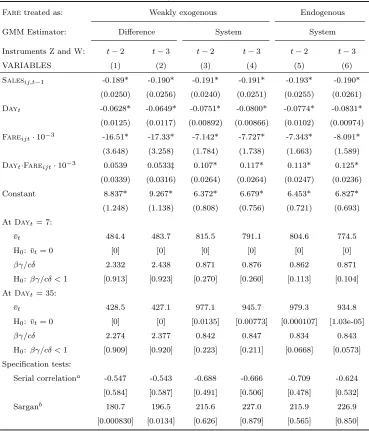
The estimation results are presented in Table 1. Fareijt is treated as weakly exogenous
in columns 1 through 4 and as endogenous in columns 5 and 6. All system GMM
specifi-cations pass both identification tests: there is no serial correlation in εijt and the Sargan
test validates the instrument lists. The negative and statistically significant coefficient on
Dayt across all specifications indicates that the number of active consumers Nt increases
as the departure date approaches — using the point estimates in the last column we find
that Nt increases from 3.47 at Dayt = 35 to 5.59 at Dayt = 7.5 In addition, we have a
4
The conditionβγ/cδ <1 is obtained from∂¯vt/∂Dayt>0. 5
downward sloping demand — at the sample mean of Dayt, a one dollar increase in fares
decreases sales by 0.155 seats in a 100-seat aircraft.
[Table 1, here.]
The estimates in the last column show that the highest valuation for an airline seat
at 35 days to departure is $934.8 while it is $774.5 at 7 days to departure. Both of
these figures are statistically significant as shown by the small p-values associated with the
null that the population parameters are equal to zero. Smaller estimates of ¯v closer to
departure are also found across all system GMM specifications under different assumptions
on the contemporaneous correlation betweenFareijtandεijt, and with different lags in the
instrument vectorsZand W. When looking at the condition to have decreasing valuations
we have that the estimates of βγ/cδ are 0.843 and 0.871 at 35 and 7 days to departure
respectively. The p-values associated with the null of βγ/cδ < 1 indicate that at a 10%
significance level we reject the null of decreasing valuations at 7 days to departure, but we
fail to reject the null at 35 days to departure.6
Note that this simple dynamic demand structure assumes that 1) valuations at time t
are uniformly distributed, 2) only ¯vt changes with t, not the lower bound or the shape of
the distribution, and 3) consumers purchase immediately and vanish otherwise.
Assump-tions one and two help define a linear demand that rotates clockwise as ¯vt increases. The
specification of a linear demand implies that changes in the demand intercept ¯v as time to
departure declines are identified by changes in the slope of the demand as time to departure
declines. While the demand estimation allows consumers to behave dynamically,
assump-tion three and the identificaassump-tion of ¯v comes from a simple demand specification where
consumers cannot choose when to purchase. Our estimates cannot distinguish between
consumers with low valuations arriving late and those with low valuations postponing their
purchase decisions.
A more general dynamic demand interpretation follows from Deneckere and Peck (2012)’s
model in which consumers can choose when to purchase. Our results can also be interpreted
as the average value of the fixed effects) and lagged fitted values forSalest−1, obtained assuming that all
previous shocksεt are zero. The regression constant affectsNt and ¯vtviac. 6
If we restrictNt to be constant (i.e., β= 0), the condition for decreasing valuations is simply δ >0,
as showing that consumers wait if time to departure is high but not if time to departure
is low. That is, if consumers with the same distribution of valuations arrive in random
order, the option to wait makes early consumers (particularly those with low valuations)
less sensitive to price. Then as time goes by the distribution of remaining consumers will
become more skewed towards lower valuations. As the option of waiting declines these
consumers will start to act more price sensitive, consistent with our results.
6
Conclusion
Our results support the claim that consumers’ purchasing behavior changes as the
depar-ture date nears. When we view consumers as making instantaneous decisions, the evidence
suggests that they become more price sensitive as the time to departure draws closer which
is consistent with having lower valuations. High-valuation consumers buying earlier is
con-sistent with one key prediction in Deneckere and Peck (2012). Our result can be interpreted
as evidence that airline travelers sort themselves efficiently in equilibrium with low
valua-tion types postponing their purchase decisions and even deciding not to buy if prices closer
to departure are higher than their valuation. Deneckere and Peck (2012) explain that this
implies that rationing arises endogenously in equilibrium. While their model predicts that
markets clear, airline markets still show underutilized capacity that perhaps arises due
to high aggregate demand uncertainty, price stickiness, or slow or incomplete aggregate
demand learning.
References
Alderighi, M., 2010. Fare dispersions in airline markets: A quantitative assessment of
theoretical explanations.Journal of Air Transport Management 16, 144-150.
Alderighi, M., M. Nicolini, and C.A. Piga, 2012. Combined Effects of Load Factors and
Booking Time on Fares: Insights from the Yield Management of a Low-Cost Airline.
FEEM Working Paper.
evidence and an application to employment equations.Review of Economic Studies 58,
277-297.
Bieger, T., A. Wittmer, and C. Laesser, 2007. What is driving the continued growth in
demand for air travel? Customer value of air transport.Journal of Air Transport
Man-agement13, 31-36.
Bitran, G.R. and S.V. Mondschein, 1997. Periodic pricing of seasonal product in retailing.
Management Science43, 64-79.
Baltagi, B.H., 2013.Econometrics Analysis of Panel Data. 5th ed. Chichester, UK: Wiley.
Baltagi, B.H. and D. Levin, 1986. Estimating dynamic demand for cigarettes using panel
data: The effects of bootlegging, taxation and advertising reconsidered.Review of
Eco-nomics and Statistics68, 148-155.
Bilotkach, B., Y. Gorodnichenkob, and O. Talavera, 2010. Are airlines’ price-setting
strate-gies different? Journal of Air Transport Management16, 1-6.
Bilotkach, V. and N. Rupp, 2011. A guide to booking airline tickets online. in James Peoples
(ed.)Pricing Behavior and Non-Price Characteristics in the Airline Industry (Advances
in Airline Economics, Volume 3), Emerald Group Publishing Limited, 83-105.
Blundell, R.W. and S. Bond, 1998. Initial conditions and moment restrictions in dynamic
panel data models.Journal of Econometrics87, 115-143.
Brons, M., E. Pels, P. Nijkamp, and P. Rietveld, 2002. Price elasticities of demand for
passenger air travel: a meta-analysis.Journal of Air Transport Management8, 165-175.
Chevalier, J.A. and A.K. Kashyap, 2011. Best prices. NBER working paper 16680.
Cam-bridge, MA.
DHaultfœuille X., P. F´evrier, and L. Wilner, 2013. Demand estimation in the presence of
revenue management. Working Paper.
Dana, Jr. J., 1998. Advance-purchase discounts and price discrimination in competitive
Deneckere, R. and J. Peck, 2011. Dynamic competition with random demand and costless
search: A theory of price posting.Econometrica80, 1185-1247.
Escobari, D., 2009. Systematic peak-load pricing, congestion premia and demand diverting:
Empirical evidence.Economics Letters103, 59-61.
Escobari, D., 2012. Dynamic pricing, advance sales, and aggregate demand learning in
airlines.Journal of Industrial Economics60, 697-724.
Escobari, D. and P. Jindapon, 2014. Price discrimination through refund contracts in
air-lines.International Journal of Industrial Organization, 34, pp. 1-8.
Escobari, D., N. Rupp., and J. Meskey, 2013. Dynamic price discrimination in airlines.
Working Paper.
Gale, I. and T. Holmes, 1993. Advance-purchase discounts and monopoly allocation of
capacity.American Economic Review83, 135-146.
Gallego, G. and G.J. van Ryzin, 1994. Optimal dynamic pricing of inventories with
stochas-tic demand over finite horizons.Management Science40, 999-1020.
Ito, H. and D. Lee, 2005. Assessing the impact of the September 11 terrorist attacks on
U.S. airline demand.Journal of Economics and Business57, 75-96.
Lazarev, J., 2013. The welfare effects of intertemporal price discrimination: An empirical
analysis of airline pricing in U.S. mononoly markets. Working Paper.
Lederman, M., 2007. Do enhancements to loyalty programs affect demand? The impact of
international frequent flyer partnerships on domestic airline demand.RAND Journal of
Economics38, 1134-1158.
Malighetti, P., S. Paleari, and R. Redondi, 2009. Pricing strategies of low-cost airlines: The
Ryanair case study.Journal of Air Transport Management 15, 195-203.
Mantin, B. and B. Koo, 2009. Dynamic price dispersion in airline markets.Transportation
McAfee, R. P. and V. te Velde, 2007. Dynamic pricing in the airline industry. In Hendershott
T. J. (ed.), Handbook of Economics and Information Systems, Vol. 1, (Elsevier Science,
New York, New York, U.S.A.).
Nevo, A. and I. Hendel, 2013. Intertemporal price discrimination in storable goods markets.
American Economic Review 103, 2722-2751.
Siegert, C. and R. Ulbricht, 2014. Dynamic oligopoly pricing: Evidence from the airline
industry. Working Paper.
Stokey, N.L., 1979. Intertemporal price discrimination.Quarterly Journal of Economics93,
355-371.
Stavins, J., 2001. Price discrimination in the airline market: The effect of market
concen-tration.Review of Economics and Statistics 83, 200-202.
Vulcano, G., G. van Ryzin, and W. Chaar, 2010. Choice-based revenue management: An
empirical study of estimation and optimization. Manufacturing & Service Operations
Management12, 375-388.
Wei, W. and M. Hansen, 2005. Impact of aircraft size and seat availability on airlines
demand and market share in duopoly markets.Transportation Research Part E41,
315-327.
Williams, K.R., 2013. Dynamic Airline Pricing and Seat Availability. Working Paper.
Yan, S. and C-H. Tseng, 2002. A passenger demand model for airline flight scheduling and
fleet routing.Computers & Operations Research 29, 1559-1581.
Zhao, W. and Y.S. Zheng, 2000. Optimal dynamic pricing for perishable assets with
Table 1: GMM Dynamic Demand Results
Faretreated as: Weakly exogenous Endogenous
GMM Estimator: Difference System System
InstrumentsZandW: t−2 t−3 t−2 t−3 t−2 t−3
VARIABLES (1) (2) (3) (4) (5) (6)
Salesij,t−1 -0.189* -0.190* -0.191* -0.191* -0.193* -0.190*
(0.0250) (0.0256) (0.0240) (0.0251) (0.0255) (0.0261)
Dayt -0.0628* -0.0649* -0.0751* -0.0800* -0.0774* -0.0831*
(0.0125) (0.0117) (0.00892) (0.00866) (0.0102) (0.00974)
Fareijt·10−3
-16.51* -17.33* -7.142* -7.727* -7.343* -8.091* (3.648) (3.258) (1.784) (1.738) (1.663) (1.589)
Dayt·Fareijt·10−3
0.0539 0.0533‡ 0.107* 0.117* 0.113* 0.125*
(0.0339) (0.0316) (0.0264) (0.0264) (0.0247) (0.0236) Constant 8.837* 9.267* 6.372* 6.679* 6.453* 6.827*
(1.248) (1.138) (0.808) (0.756) (0.721) (0.693) AtDayt = 7:
¯
vt 484.4 483.7 815.5 791.1 804.6 774.5
H0: ¯vt= 0 [0] [0] [0] [0] [0] [0]
βγ/cδ 2.332 2.438 0.871 0.876 0.862 0.871
H0:βγ/cδ <1 [0.913] [0.923] [0.270] [0.260] [0.113] [0.104]
AtDayt = 35: ¯
vt 428.5 427.1 977.1 945.7 979.3 934.8
H0: ¯vt= 0 [0] [0] [0.0135] [0.00773] [0.000107] [1.03e-05]
βγ/cδ 2.274 2.377 0.842 0.847 0.834 0.843
H0:βγ/cδ <1 [0.909] [0.920] [0.223] [0.211] [0.0668] [0.0573]
Specification tests:
Serial correlationa -0.547 -0.543 -0.688 -0.666 -0.709 -0.624
[0.584] [0.587] [0.491] [0.506] [0.478] [0.532] Sarganb 180.7 196.5 215.6 227.0 215.9 226.9
[0.000830] [0.0134] [0.626] [0.879] [0.565] [0.850]
Notes: The dependent variable is Salesijt. Figures in parentheses are the Windmeijer finite-sample corrected standard errors of the GMM two-step estimates. ‡significant at 10%;†significant at 5%; ∗
significant at 1%. Figures in square brackets are p-values. a The null hypothesis is that the errors in
the first-difference regression exhibit no second-order serial correlation (valid specification). bThe null