Using N-gram and Word Network Features for
Native Language Identification
Shibamouli Lahiri Rada Mihalcea Computer Science and Engineering
University of North Texas Denton, TX 76207, USA
[email protected], [email protected]
Abstract
We report on the performance of two different feature sets in the Native Language Identification Shared Task (Tetreault et al., 2013). Our feature sets were inspired by existing literature on native language identification and word networks. Exper-iments show that word networks have competitive performance against the baseline feature set, which is a promising result. We also present a discussion of feature analysis based on information gain, and an overview on the performance of different word net-work features in the Native Language Identification task.
1 Introduction
Native Language Identification (NLI) is a well-established problem in NLP, where the goal is to identify a writer’s native language (L1) from his/her writing in a second language (L2), usually English. NLI is generally framed as a multi-class classifi-cation problem (Koppel et al., 2005; Brooke and Hirst, 2011; Wong and Dras, 2011), where native languages (L1) are considered class labels, and writ-ing samples in L2 are used as trainwrit-ing and test data. The NLI problem has recently seen a big surge in interest, sparked in part by three influential early pa-pers on this problem (Tomokiyo and Jones, 2001; van Halteren and Oostdijk, 2004; Koppel et al., 2005). Apart from shedding light on the way non-native learners (also called “L2 learners”) learn a new language, the NLI task allows constrastive anal-ysis (Wong and Dras, 2009), study of different types
of errors that people make while learning a new lan-guage (Kochmar, 2011; Bestgen et al., 2012; Jarvis et al., 2012), and identification of language trans-fer patterns (Brooke and Hirst, 2012a; Jarvis and Crossley, 2012), thereby helping L2-students im-prove their writing styles and expediting the learn-ing process. It also helps L2 educators to concen-trate their efforts on particular areas of a language that cause the most learning difficulty for different L1s.
The NLI task is closely related to traditional NLP problems of authorship attribution (Juola, 2006; Sta-matatos, 2009; Koppel et al., 2009) and author pro-filing (Keˇselj et al., 2003; Estival et al., 2007a; Esti-val et al., 2007b; Bergsma et al., 2012), and shares many of the same features. Like authorship attri-bution, NLI is greatly benefitted by having function words and character n-grams as features (Brooke and Hirst, 2011; Brooke and Hirst, 2012b). Native languages form a part of an author’s socio-cultural and psychological profiles, thereby being related to author profiling (van Halteren and Oostdijk, 2004; Torney et al., 2012).
Researchers have used different types of features for the NLI problem, including but not limited to function words (Brooke and Hirst, 2012b); char-acter, word and POS n-grams (Brooke and Hirst, 2012b); spelling and syntactic errors (Koppel et al., 2005); CFG productions (Brooke and Hirst, 2012b); Tree Substitution Grammar productions (Swanson and Charniak, 2012); dependencies (Brooke and Hirst, 2012b); Adaptor Grammar features (Wong et al., 2012); L1-influence (Brooke and Hirst, 2012a); stylometric features (Golcher and Reznicek, 2011;
Crossley and McNamara, 2012; Jarvis et al., 2012); recurrent n-grams on words and POS (Bykh and Meurers, 2012); and features derived from topic models (Wong et al., 2011). State-of-the-art sults are typically in the 80%-90% range, with re-sults above 90% reported in some cases (Brooke and Hirst, 2012b). Note, however, that results vary greatly across different datasets, depending on the number of languages being considered, size and dif-ficulty of data, etc.
2 Our Approach
The NLI 2013 Shared Task (Tetreault et al., 2013) marks an effort in bringing together the NLI research community to share and compare their results and evaluations on a common dataset - TOEFL11 (Blan-chard et al., 2013) - consisting of 12,100 unique En-glish essays written by non-native learners of eleven different languages.1 The dataset has 9,900 essays for training, 1,100 essays for test, and 1,100 essays for development. Each of the three sets is balanced across different L1s.
Inspired by previous work in NLI, in our different NLI systems submissions we used several different types of character, word, and POS n-gram features (cf. Section 2.1). Although not included in the sys-tems submitted, we also experimented with a family of new features derived from a word network repre-sentation of natural language text (cf. Section 2.2). We used Weka (Hall et al., 2009) for all our classifi-cation experiments. The systems that were submit-ted gave best 10-fold cross-validation accuracy on training data among different feature-classifier com-binations (Section 3). Word network features - al-though competitive against the baseline n-gram fea-tures - were not able to beat the baseline feafea-tures on the training set, so we did not submit that sys-tem for evaluation. Section 2.1 discusses our n-gram features, followed by a discussion of word network features in Section 2.2.
2.1 N-gram Features
We used several baseline n-gram features based on words, characters, and POS. We experimented with the raw frequency, normalized frequency, and binary
1Arabic, Chinese, French, German, Hindi, Italian, Japanese,
Korean, Spanish, Telugu and Turkish.
presence/absence indicator on top 100, 200, 500 and 1000 n-grams:2
1. word n-grams (n = 1, 2, 3), with and without punctuation.
2. character n-grams (n = 1, 2, 3), with and with-out space characters.
3. POS n-grams (n = 1, 2, 3), with and without punctuation.3
We experimented with punctuation because pre-vious research indicates that punctuation is help-ful (Wong and Dras, 2009; Kochmar, 2011). In total, there are 216 types of n-gram feature vectors (with dimensions 100, 200, 500 and 1000) for a particular document. Because of size restrictions (e.g., some n-gram dictionaries are smaller than the specified fea-ture vector dimensions), we ended up with 168 types of feature vectors per document (cf. Tables 2 to 4).
2.2 Word Networks
A “word network” of a particular document is a net-work (graph) of unique words found in that docu-ment. Each node (vertex) in this network is a word. Edges between two nodes (unique words) can be constructed in several different ways. The simplest type of edge connects word A to word B, if word A is followed by word B in the document at least once. In our work, we have assumed a directed edge with direction from word A to word B. Note that we could have used undirected edges as well (cf. (Mi-halcea and Tarau, 2004)). Moreover, edges can be weighted/unweighted. We assumed unweighted edges.
A deeper issue with this network construction process concerns what we should do with stopwords. Should we keep them, or should we remove them? Since stopwords and function words have proved to be of special importance in previous native language identification studies (Wong and Dras, 2009; Brooke and Hirst, 2012b), we chose to keep them in our word networks.
Two other choices we made in the construction of our word networks concern sentence boundaries
2Note that these most frequent n-grams were extracted from
the training+development set.
3
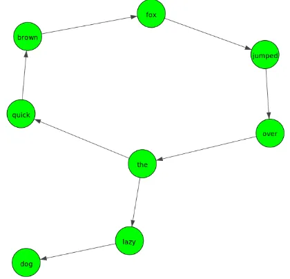
Figure 1: Word network of the sentence“the quick brown fox jumped over the lazy dog”.
and word co-occurrence. Word networks can be constructed either by respecting sentence boundaries (where the last word of sentence 1 does not link to the first word of sentence 2), or by disregard-ing them. In our case, we disregarded all sentence boundaries. Moreover, a network edge can either link two words that appeared side-by-side in the original document, or it can link two words that ap-peared within a window ofnwords in the document (cf. (Mihalcea and Tarau, 2004)). In our case, we chose the first option - linking unique words that ap-peared side-by-side at least once. Finally, we did not perform any stemming/morphological analysis to retain subtle cues that might be revealed from in-flected/derived words.
The word network of an example sentence (“the quick brown fox jumped over the lazy dog”) is shown in Figure 1. Note that the word “the” ap-peared twice in this sentence, so the correspond-ing network contains a cycle that starts at “the” and ends at “the”. In a realistic word network of a large document, there can be many such cycles. In addition, it is observed that such word networks show power-law degree distribution and a small-world structure (i Cancho and Sol´e, 2001; Matsuo et al., 2001).
Once the word networks have been constructed, we extract a set of simple features from these
net-works4 that represent local properties of individual nodes. We have extracted ten local features for each node in a word network:
1. in-degree, out-degree and degree
2. in-coreness, out-coreness and coreness5
3. in-neighborhood size (order 1), out-neighborhood size (order 1) and out-neighborhood size (order 1)
4. local clustering coefficient
We take a set ofrepresentative words, and convert a document into a local feature vector - each local feature pertaining to one word in the set of repre-sentative words. For example, when we use the top 200 most frequent words as the representative set, a document can be represented as the degree vec-tor of these 200 words in the document’s word net-work, or as the local clustering coefficient vector of these words in the word network, or as the coreness vector of the words (and so on). A document can also be represented as a concatenation (mixture) of these vectors. For example, it can be represented
asconcat(degree vector, coreness vector)of top
200 most frequent words. We are yet to explore how such mixed feature sets perform in the NLI task, and this constitutes a part of our future work (Section 4). We experimented with top k most fre-quent words (with k = 100, 200, 500, 1000) on train-ing+development data as our representative word-set.
3 Results
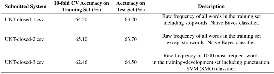
Table 1 describes the three systems we submitted. The first two systems (UNT-closed-1.csv and UNT-closed-2.csv) were based on a bag of words model using all the words from the training set. The systems used a home-grown implementation of the Na¨ıve Bayes classifier, and achieved 10-fold cross-validation accuracy of 64.5% and 65.1% respec-tively, on the training set. The first system used raw
4
We used the igraph (Csardi and Nepusz, 2006) software package for graph feature extraction.
5
Submitted System 10-fold CV Accuracy on Accuracy on Description
Training Set (%) Test Set (%)
UNT-closed-1.csv 64.50 63.20 Raw frequency of all words in the training set including stopwords. Na¨ıve Bayes classifier.
UNT-closed-2.csv 65.10 63.70 Raw frequency of all words in the training set except stopwords. Na¨ıve Bayes classifier.
UNT-closed-3.csv 62.46 64.50
Raw frequency of 1000 most frequent words in the training+development set including punctuation.
[image:4.612.77.533.58.182.2]SVM (SMO) classifier.
Table 1: Performance summary and description of the systems we submitted.
term frequency of all words including stopwords as features, and the second system used raw term fre-quency of all words except stopwords. These two systems achieved test set accuracy of 63.2% and 63.7%, respectively.
The third system we submitted ( UNT-closed-3.csv) was based on n-gram features (cf. Sec-tion 2.1). We used the raw frequency of top 1000 word unigrams, including punctuation, as features. The Weka SMO implementation of SVM (Hall et al., 2009) was used as classifier with default param-eter settings. This system gave us the best 10-fold cross-validation accuracy of 62.46% in the training set, among all n-gram features. Note that this system was also the top performer among the systems we submitted in NLI evaluation, with a test set accuracy of 64.5%, and a 10-fold CV accuracy of 63.77% on the training+development set folds specified by the organizers.
We will now describe in the following two sub-sections how our n-gram features and word network features performed on the training set. All results re-ported here reflect best 10-fold cross-validation ac-curacy in the training set among different classifiers (SVM, Na¨ıve Bayes, 1-nearest-neighbor (1NN), J48 decision tree, and AdaBoost). SVM and Na¨ıve Bayes gave best results in our experiments, so only these two are shown in Tables 2 to 5.
3.1 Performance of N-gram Features
Recall from Section 2.1 that we extracted 168 differ-ent n-gram feature vectors corresponding to the raw frequency, normalized frequency, and binary pres-ence/absence indicator of top k n-grams (withk = 100, 200, 500, 1000) in the training+development
set. Performance of these n-gram features is given in Tables 2 to 4. A general observation with Tables 2 to 4 is that cross-validation performance improves as
kincreases, although there are a few exceptions. We marked those exceptions with an asterisk (“*”).
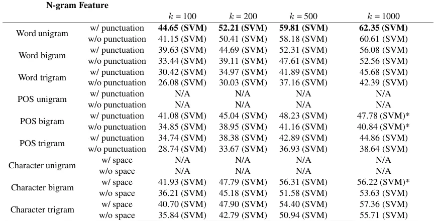
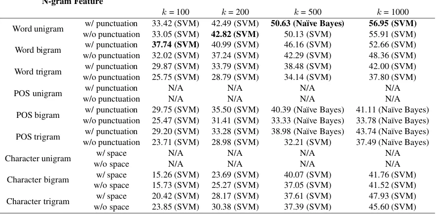
It is interesting to note that topkword unigrams with punctuation were the top performers in most of the cases. Also interesting is the fact that SVM mostly gave best performance on n-gram features among different classifiers. Note that Na¨ıve Bayes was best performer in a few cases (Table 4). Per-formance of raw and normalized frequency features were mostly comparable (Tables 2 and 3), whereas binary presence/absence indicator achieved worse accuracy values in general than raw and normalized frequency features (Table 4).
Among different n-grams, word unigrams per-formed better than bigrams and trigrams, POS bi-grams performed better than POS tribi-grams, and character bigrams and character trigrams performed comparably well (Tables 2 and 3). Exceptions to this observation are seen in Table 4, where character trigrams performed better than character bigrams, and word bigrams sometimes performed better than word unigrams. In general, word n-grams performed the best, followed by POS and character n-grams.
3.2 Performance of Word Network Features
per-N-gram Feature
Best Cross-validation Accuracy (%) on TopkMost Frequent N-grams
k= 100 k= 200 k= 500 k= 1000
Word unigram w/ punctuation 45.07 (SVM) 52.85 (SVM) 60.14 (SVM) 62.46 (SVM) w/o punctuation 41.63 (SVM) 50.15 (SVM) 58.33 (SVM) 60.85 (SVM)
Word bigram w/ punctuation 39.54 (SVM) 44.75 (SVM) 51.70 (SVM) 56.06 (SVM) w/o punctuation 33.40 (SVM) 39.34 (SVM) 47.54 (SVM) 51.86 (SVM)
Word trigram w/ punctuation 30.62 (SVM) 35.26 (SVM) 41.56 (SVM) 44.97 (SVM) w/o punctuation 26.67 (SVM) 30.14 (SVM) 36.68 (SVM) 41.22 (SVM)
POS unigram w/ punctuation N/A N/A N/A N/A
w/o punctuation N/A N/A N/A N/A
POS bigram w/ punctuation 41.79 (SVM) 45.87 (SVM) 48.11 (SVM) 47.49 (SVM)* w/o punctuation 35.95 (SVM) 39.23 (SVM) 41.23 (SVM) 39.58 (SVM)*
POS trigram w/ punctuation 34.97 (SVM) 38.78 (SVM) 43.17 (SVM) 44.52 (SVM) w/o punctuation 29.73 (SVM) 34.31 (SVM) 37.58 (SVM) 38.40 (SVM)
Character unigram w/ space N/A N/A N/A N/A
w/o space N/A N/A N/A N/A
Character bigram w/ space 42.48 (SVM) 48.43 (SVM) 55.87 (SVM) 56.12 (SVM) w/o space 36.84 (SVM) 45.93 (SVM) 51.11 (SVM) 53.41 (SVM)
[image:5.612.91.522.92.308.2]Character trigram w/ space 41.65 (SVM) 48.68 (SVM) 54.54 (SVM) 57.77 (SVM) w/o space 36.64 (SVM) 43.44 (SVM) 51.46 (SVM) 55.52 (SVM)
Table 2: Performance of raw frequency of n-gram features. Stratified ten-fold cross-validation accuracy values on TOEFL11 training set are shown, along with the classifiers that achieved these accuracy values. Best results in different columns are boldfaced. Table cells marked “N/A” are the ones that correspond to an n-gram dictionary size< k.
N-gram Feature
Best Cross-validation Accuracy (%) on TopkMost Frequent N-grams
k= 100 k= 200 k= 500 k= 1000
Word unigram w/ punctuation 44.65 (SVM) 52.21 (SVM) 59.81 (SVM) 62.35 (SVM) w/o punctuation 41.15 (SVM) 50.41 (SVM) 58.18 (SVM) 60.61 (SVM)
Word bigram w/ punctuation 39.63 (SVM) 44.69 (SVM) 52.31 (SVM) 56.08 (SVM) w/o punctuation 33.44 (SVM) 39.11 (SVM) 47.61 (SVM) 52.56 (SVM)
Word trigram w/ punctuation 30.42 (SVM) 34.97 (SVM) 41.89 (SVM) 45.68 (SVM) w/o punctuation 26.08 (SVM) 30.03 (SVM) 37.16 (SVM) 42.39 (SVM)
POS unigram w/ punctuation N/A N/A N/A N/A
w/o punctuation N/A N/A N/A N/A
POS bigram w/ punctuation 41.08 (SVM) 45.04 (SVM) 48.23 (SVM) 47.78 (SVM)* w/o punctuation 34.85 (SVM) 38.95 (SVM) 41.16 (SVM) 40.84 (SVM)*
POS trigram w/ punctuation 34.74 (SVM) 38.38 (SVM) 42.89 (SVM) 44.86 (SVM) w/o punctuation 28.74 (SVM) 33.67 (SVM) 36.93 (SVM) 38.64 (SVM)
Character unigram w/ space N/A N/A N/A N/A
w/o space N/A N/A N/A N/A
Character bigram w/ space 41.93 (SVM) 47.79 (SVM) 56.31 (SVM) 56.22 (SVM)* w/o space 36.21 (SVM) 45.18 (SVM) 51.58 (SVM) 53.63 (SVM)
Character trigram w/ space 40.70 (SVM) 47.90 (SVM) 54.40 (SVM) 57.36 (SVM) w/o space 35.84 (SVM) 42.79 (SVM) 50.94 (SVM) 55.71 (SVM)
Table 3: Performance of normalized frequency of n-gram features. Stratified ten-fold cross-validation accuracy values on TOEFL11 training set are shown, along with the classifiers that achieved these accuracy values. Best results in different columns are boldfaced. Table cells marked “N/A” are the ones that correspond to an n-gram dictionary size
[image:5.612.89.522.409.629.2]N-gram Feature
Best Cross-validation Accuracy (%) on TopkMost Frequent N-grams
k= 100 k= 200 k= 500 k= 1000
Word unigram w/ punctuation 33.42 (SVM) 42.49 (SVM) 50.63 (Na¨ıve Bayes) 56.95 (SVM) w/o punctuation 33.05 (SVM) 42.82 (SVM) 50.13 (SVM) 55.91 (SVM)
Word bigram w/ punctuation 37.74 (SVM) 40.99 (SVM) 46.16 (SVM) 52.66 (SVM) w/o punctuation 32.02 (SVM) 37.24 (SVM) 42.29 (SVM) 48.36 (SVM)
Word trigram w/ punctuation 29.87 (SVM) 33.79 (SVM) 38.48 (SVM) 42.00 (SVM) w/o punctuation 25.75 (SVM) 28.79 (SVM) 34.14 (SVM) 37.80 (SVM)
POS unigram w/ punctuation N/A N/A N/A N/A
w/o punctuation N/A N/A N/A N/A
POS bigram w/ punctuation 29.75 (SVM) 35.50 (SVM) 40.39 (Na¨ıve Bayes) 41.11 (Na¨ıve Bayes) w/o punctuation 25.47 (SVM) 31.41 (SVM) 33.33 (Na¨ıve Bayes) 33.78 (Na¨ıve Bayes)
POS trigram w/ punctuation 29.20 (SVM) 33.28 (SVM) 38.98 (Na¨ıve Bayes) 43.74 (Na¨ıve Bayes) w/o punctuation 23.71 (SVM) 28.98 (SVM) 32.21 (SVM) 37.49 (Na¨ıve Bayes)
Character unigram w/ space N/A N/A N/A N/A
w/o space N/A N/A N/A N/A
Character bigram w/ space 15.26 (SVM) 23.69 (SVM) 40.07 (SVM) 41.76 (SVM) w/o space 15.73 (SVM) 25.27 (SVM) 37.05 (SVM) 41.52 (SVM)
[image:6.612.86.528.104.321.2]Character trigram w/ space 20.42 (SVM) 28.17 (SVM) 37.61 (SVM) 47.93 (SVM) w/o space 23.85 (SVM) 30.38 (SVM) 37.39 (SVM) 45.60 (SVM)
Table 4: Performance of binary presence/absence indicator on n-gram features. Stratified ten-fold cross-validation accuracy values on TOEFL11 training set are shown, along with the classifiers that achieved these accuracy values. Best results in different columns are boldfaced. Table cells marked “N/A” are the ones that correspond to an n-gram dictionary size< k.
Word Network Feature
Best Cross-validation Accuracy (%) on TopkMost Frequent Words
k= 100 k= 200 k= 500 k= 1000
Clustering Coefficient 15.31 (SVM) 17.73 (SVM) 19.96 (SVM) 20.71 (SVM) In-degree 39.89 (SVM) 49.28 (SVM) 56.83 (SVM) 59.47 (SVM) Out-degree 40.66 (SVM) 49.67 (SVM) 57.16 (SVM) 59.62 (SVM) Degree 41.05 (SVM) 50.74 (SVM) 58.17 (SVM) 60.21 (SVM) In-coreness 32.52 (SVM) 42.44 (SVM) 51.09 (SVM) 55.50 (SVM) Out-coreness 32.41 (SVM) 43.15 (SVM) 51.34 (SVM) 55.39 (SVM) Coreness 35.32 (SVM) 45.84 (SVM) 53.54 (SVM) 57.18 (SVM) In-neighborhood Size
40.54 (SVM) 50.08 (SVM) 56.92 (SVM) 59.69 (SVM) (order 1)
Out-neighborhood Size
41.09 (SVM) 50.09 (SVM) 57.71 (SVM) 59.73 (SVM) (order 1)
Neighborhood Size
41.83 (SVM) 50.68 (SVM) 57.40 (SVM) 60.41 (SVM)
(order 1)
Rank Word Network Feature Information Gain
1 Degree of the worda 0.1058
2 Neighborhood size of the worda 0.1054 3 Out-neighborhood size of the worda 0.1050
4 Outdegree of the worda 0.1049
5 In-neighborhood size of the worda 0.1017
6 Indegree of the worda 0.1016
7 Neighborhood size of the wordhowever 0.0928
8 Degree of the wordhowever 0.0928
9 Indegree of the wordhowever 0.0928
10 In-neighborhood size of the wordhowever 0.0928 11 Outdegree of the wordhowever 0.0916 12 Out-neighborhood size of the wordhowever 0.0916 13 Out-coreness of the wordhowever 0.0851 14 Coreness of the wordhowever 0.0851 15 In-coreness of the wordhowever 0.0850
16 Outdegree of the wordthe 0.0793
17 Out-neighborhood size of the wordthe 0.0790
18 Degree of the wordthe 0.0740
19 Neighborhood size of the wordthe 0.0740
[image:7.612.164.448.55.289.2]20 Coreness of the worda 0.0710
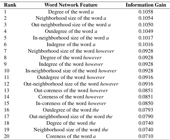
Table 6: Ranking of word network features based on Information Gain, on TOEFL11 training set. We took 1000 most frequent words on the training+development set, and collected all their word network features in a single file. This ranking reflects the top 20 features in that file, along with their information gain values.
formed quite well, with the best result (60.41% CV accuracy on the train set) being competitive against (but slightly worse than) the baseline n-gram fea-tures (62.46% CV accuracy on the train set). Perfor-mance improved with increasingk, thereby corrob-orating our general observation from Tables 2 to 4. Clustering coefficient performed poorly, and seems rather unsuitable for the NLI task. But degree, core-ness, and neighborhood size performed good. Here also, SVM turned out to be the best classifier, giving best CV accuracy in all cases.
We experimented with the in-, out-, and over-all versions of degree, coreness and neighborhood size. Their performance was mostly comparable with each other (Table 5). To investigate which word network features are the most discriminatory in this task, we collected all ten word network features of the top 1000 words in a single file, and then ranked those features on the training set based on Infor-mation Gain (IG). The 20 top-ranking features are shown in Table 6, along with their corresponding IG values. Note that the wordsa,the, andhowever
were among the most discriminatory, and different versions of degree, neighborhood size and coreness appeared among the top, which is in line with our
earlier observation that clustering coefficients were not very discriminatory at the native language clas-sification task.
4 Conclusions and Future Work
In this paper, we described experiments with the NLI task using a baseline set of n-gram features, and a set of novel features derived from a word network representation of text documents. Useful and less useful n-gram features were identified, along with the fact that SVM was the best classifier in most of the cases. We learned that when using raw or normalized frequency, lower-order n-grams perform at least as good as higher-order n-grams; moreover, Na¨ıve Bayes sometimes give good results when bi-nary presence/absence indicator variables are used as features.
gain helped us identify the most important word net-work features in a collection of top 1000 words in the training+development set.
Future work consists of experimenting with com-bined word network features; mixed word network features and baseline n-gram features; and the one-vs-all classification scheme instead of the multiclass classification scheme.
References
Vladimir Batagelj and Matjaz Zaversnik. 2003. An O(m) Algorithm for Cores Decomposition of Net-works. CoRR, cs.DS/0310049.
Shane Bergsma, Matt Post, and David Yarowsky. 2012. Stylometric Analysis of Scientific Articles. In Pro-ceedings of the 2012 Conference of the North Ameri-can Chapter of the Association for Computational Lin-guistics: Human Language Technologies, pages 327– 337, Montr´eal, Canada, June. Association for Compu-tational Linguistics.
Yves Bestgen, Sylviane Granger, and Jennifer Thewis-sen. 2012. Error Patterns and Automatic L1 Identifi-cation. In Scott Jarvis and Scott A. Crossley, editors, Approaching Language Transfer through Text Classi-fication, pages 127–153. Multilingual Matters. Daniel Blanchard, Joel Tetreault, Derrick Higgins, Aoife
Cahill, and Martin Chodorow. 2013. TOEFL11: A Corpus of Non-Native English. Technical report, Ed-ucational Testing Service.
Julian Brooke and Graeme Hirst. 2011. Native language detection with ‘cheap’ learner corpora. InConference of Learner Corpus Research (LCR2011), Louvain-la-Neuve, Belgium. Presses universitaires de Louvain. Julian Brooke and Graeme Hirst. 2012a. Measuring
Interlanguage: Native Language Identification with L1-influence Metrics. In Nicoletta Calzolari, Khalid Choukri, Thierry Declerck, Mehmet U˘gur Do˘gan, Bente Maegaard, Joseph Mariani, Jan Odijk, and Ste-lios Piperidis, editors, Proceedings of the Eighth In-ternational Conference on Language Resources and Evaluation (LREC-2012), pages 779–784, Istanbul, Turkey, May. European Language Resources Associ-ation (ELRA). ACL Anthology Identifier: L12-1016. Julian Brooke and Graeme Hirst. 2012b. Robust,
Lex-icalized Native Language Identification. In Proceed-ings of COLING 2012, pages 391–408, Mumbai, In-dia, December. The COLING 2012 Organizing Com-mittee.
Serhiy Bykh and Detmar Meurers. 2012. Native Lan-guage Identification using Recurring n-grams – In-vestigating Abstraction and Domain Dependence. In
Proceedings of COLING 2012, pages 425–440, Mum-bai, India, December. The COLING 2012 Organizing Committee.
Scott A. Crossley and Danielle McNamara. 2012. De-tecting the First Language of Second Language Writ-ers Using Automated Indices of Cohesion, Lexical Sophistication, Syntactic Complexity and Conceptual Knowledge. In Scott Jarvis and Scott A. Crossley, editors,Approaching Language Transfer through Text Classification, pages 106–126. Multilingual Matters.
Gabor Csardi and Tamas Nepusz. 2006. The igraph soft-ware package for complex network research. Inter-Journal, Complex Systems:1695.
Dominique Estival, Tanja Gaustad, Son Bao Pham, Will Radford, and Ben Hutchinson. 2007a. Author pro-filing for English emails. InProceedings of the 10th Conference of the Pacific Association for Computa-tional Linguistics, pages 263–272, Melbourne, Aus-tralia.
Dominique Estival, Tanja Gaustad, Son Bao Pham, Will Radford, and Ben Hutchinson. 2007b. TAT: An Au-thor Profiling Tool with Application to Arabic Emails. InProceedings of the Australasian Language Technol-ogy Workshop 2007, pages 21–30, Melbourne, Aus-tralia, December.
Felix Golcher and Marc Reznicek. 2011. Stylometry and the interplay of topic and L1 in the different annotation layers in the FALKO corpus. QITL-4–Proceedings of Quantitative Investigations in Theoretical Linguistics, 4:29–34.
Mark Hall, Eibe Frank, Geoffrey Holmes, Bernhard Pfahringer, Peter Reutemann, and Ian H. Witten. 2009. The WEKA data mining software: an update. SIGKDD Explor. Newsl., 11(1):10–18, November. Ramon Ferrer i Cancho and Ricard V. Sol´e. 2001. The
Small World of Human Language. Proceedings: Bio-logical Sciences, 268(1482):pp. 2261–2265.
Scott Jarvis and Scott A. Crossley, editors. 2012. Ap-proaching Language Transfer Through Text Classifica-tion: Explorations in the Detection-based Approach, volume 64. Multilingual Matters Limited, Bristol, UK.
Scott Jarvis, Yves Bestgen, Scott A. Crossley, Syl-viane Granger, Magali Paquot, Jennifer Thewissen, and Danielle McNamara. 2012. The Comparative and Combined Contributions of n-Grams, Coh-Metrix Indices and Error Types in the L1 Classification of Learner Texts. In Scott Jarvis and Scott A. Crossley, editors,Approaching Language Transfer through Text Classification, pages 154–177. Multilingual Matters.
Vlado Keˇselj, Fuchun Peng, Nick Cercone, and Calvin Thomas. 2003. N-gram-based author profiles for au-thorship attribution. InProceedings of the Conference Pacific Association for Computational Linguistics, PA-CLING, volume 3, pages 255–264.
Ekaterina Kochmar. 2011. Identification of a writer’s na-tive language by error analysis. Master’s thesis, Uni-versity of Cambridge.
Moshe Koppel, Jonathan Schler, and Kfir Zigdon. 2005. Determining an author’s native language by mining a text for errors. In Proceedings of the eleventh ACM SIGKDD international conference on Knowledge dis-covery in data mining, pages 624–628, Chicago, IL. ACM.
Moshe Koppel, Jonathan Schler, and Shlomo Argamon. 2009. Computational methods in authorship attribu-tion. J. Am. Soc. Inf. Sci. Technol., 60(1):9–26, Jan-uary.
Yutaka Matsuo, Yukio Ohsawa, and Mitsuru Ishizuka. 2001. A Document as a Small World. InProceedings of the Joint JSAI 2001 Workshop on New Frontiers in Artificial Intelligence, pages 444–448, London, UK, UK. Springer-Verlag.
Rada Mihalcea and Paul Tarau. 2004. TextRank: Bring-ing Order into Texts. In Dekang Lin and Dekai Wu, editors,Proceedings of EMNLP 2004, pages 404–411, Barcelona, Spain, July. Association for Computational Linguistics.
Xuan-Hieu Phan. 2006. CRFTagger: CRF English POS Tagger.
Efstathios Stamatatos. 2009. A survey of modern author-ship attribution methods.J. Am. Soc. Inf. Sci. Technol., 60(3):538–556, March.
Benjamin Swanson and Eugene Charniak. 2012. Na-tive Language Detection with Tree Substitution Gram-mars. InProceedings of the 50th Annual Meeting of the Association for Computational Linguistics (Vol-ume 2: Short Papers), pages 193–197, Jeju Island, Ko-rea, July. Association for Computational Linguistics. Joel Tetreault, Daniel Blanchard, and Aoife Cahill. 2013.
A Report on the First Native Language Identification Shared Task. InProceedings of the Eighth Workshop on Innovative Use of NLP for Building Educational Applications, Atlanta, GA, USA, June. Association for Computational Linguistics.
Laura Mayfield Tomokiyo and Rosie Jones. 2001. You’re not from’round here, are you?: naive Bayes de-tection of non-native utterance text. InProceedings of the second meeting of the North American Chapter of the Association for Computational Linguistics on Lan-guage technologies, pages 1–8, Pittsburgh, PA. Asso-ciation for Computational Linguistics.
Rosemary Torney, Peter Vamplew, and John Yearwood. 2012. Using psycholinguistic features for profiling
first language of authors. Journal of the Ameri-can Society for Information Science and Technology, 63(6):1256–1269.
Hans van Halteren and Nelleke Oostdijk. 2004. Linguis-tic profiling of texts for the purpose of language ver-ification. InProceedings of Coling 2004, pages 966– 972, Geneva, Switzerland, Aug 23–Aug 27. COLING. Sze-Meng Jojo Wong and Mark Dras. 2009. Contrastive Analysis and Native Language Identification. In Pro-ceedings of the Australasian Language Technology As-sociation Workshop 2009, pages 53–61, Sydney, Aus-tralia, December.
Sze-Meng Jojo Wong and Mark Dras. 2011. Exploiting Parse Structures for Native Language Identification. In Proceedings of the 2011 Conference on Empiri-cal Methods in Natural Language Processing, pages 1600–1610, Edinburgh, Scotland, UK., July. Associa-tion for ComputaAssocia-tional Linguistics.
Sze-Meng Jojo Wong, Mark Dras, and Mark Johnson. 2011. Topic Modeling for Native Language Identifi-cation. InProceedings of the Australasian Language Technology Association Workshop 2011, pages 115– 124, Canberra, Australia, December.