MSR NLP Entry in BioNLP Shared Task 2011

MSR-NLP Entry in BioNLP Shared Task 2011

Chris Quirk, Pallavi Choudhury, Michael Gamon, and Lucy Vanderwende

Microsoft Research

One Microsoft Way

Redmond, WA 98052 USA

{chrisq,pallavic,mgamon,lucyv}@microsoft.com

Abstract

We describe the system from the Natural Language Processing group at Microsoft Research for the BioNLP 2011 Shared Task. The task focuses on event extraction, identifying structured and potentially nested events from unannotated text. Our approach follows a pipeline, first decorating text with syntactic information, then identifying the trigger words of complex events, and finally identifying the arguments of those events. The resulting system depends heavily on lexical and syntactic features. Therefore, we explored methods of maintaining ambiguities and improving the syntactic representations, making the lexical information less brittle through clustering, and of exploring novel feature combinations and feature reduction. The system ranked 4th in the GENIA task with an F-measure of 51.5%, and 3rd in the EPI task with an F-measure of 64.9%.

1

Introduction

We describe a system for extracting complex events and their arguments as applied to the BioNLP-2011 shared task. Our goal is to explore general methods for fine-grained information extraction, to which the data in this shared task is very well suited. We developed our system using only the data provided for the GENIA task, but then submitted output for two of the tasks, GENIA and EPI, training models on each dataset separately, with the goal of exploring how general the overall system design is with respect to text

domain and event types. We used no external knowledge resources except a text corpus used to train cluster features. We further describe several system variations that we explored but which did not contribute to the final system submitted. We note that the MSR-NLP system consistently is among those with the highest recall, but needs additional work to improve precision.

2

System Description

Our event extraction system is a pipelined approach, closely following the structure used by the best performing system in 2009 (Björne et al., 2009). Given an input sentence along with tokenization information and a set of parses, we first attempt to identify the words that trigger complex events using a multiclass classifier. Next we identify edges between triggers and proteins, or between triggers and other triggers. Finally, given a graph of proteins and triggers, we use a rule-based post-processing component to produce events in the format of the shared task.

2.1

We began with the articles as provided, with an included tokenization of the input and identification of the proteins in the input. However, we did modify the token text and the part-of-speech tags of the annotated proteins in the input to be PROT after tagging and parsing, as we found that it led to better trigger detection.

The next major step in preprocessing was to produce labeled dependency parses for the input. Note that the dependencies may not form a tree: there may be cycles and some words may not be connected. During feature construction, this parsing graph was used to find paths between

words in the sentence. Since proteins may consist of multiple words, for paths we picked a single representative word for each protein to act as its starting point and ending point. Generally this was the token inside the protein that is closest to the root of the dependency parse. In the case of ties, we picked the rightmost such node.

2.1.1 McClosky-Charniak-Stanford parses

The organizers provide parses from a version of the McClosky-Charniak parser, MCCC (McClosky and Charniak, 2008), which is a two-stage parser/reranker trained on the GENIA corpus. In addition, we used an improved set of parsing models that leverage unsupervised data, MCCC-I (McClosky, 2010). In both cases, the Stanford Parser was used to convert constituency trees in the Penn Treebank format into labeled dependency parses: we used the collapsed dependency format.

2.1.2 Dependency posteriors

Effectively maintaining and leveraging the ambiguity present in the underlying parser has improved task accuracy in some downstream tasks (e.g., Mi et al. 2008). McClosky-Charniak parses in two passes: the first pass is a generative model that produces a set of n-best candidates, and the

second pass is a discriminative reranker that uses a rich set of features including non-local information. We renormalized the outputs from this log-linear discriminative model to get a posterior distribution over the 50-best parses. This set of parses preserved some of the syntactic ambiguity present in the sentence.

The Stanford parser deterministically converts phrase-structure trees into labeled dependency graphs (de Marneffe et al., 2006). We converted each constituency tree into a dependency graph separately and retained the probability computed above on each graph.

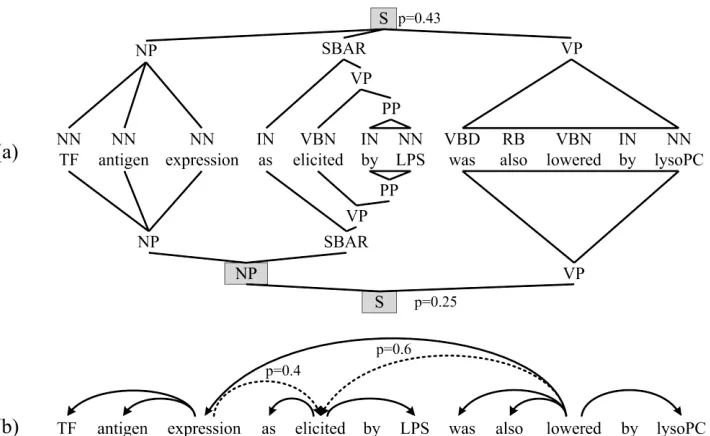
One possibility was to run feature extraction on each of these 50 parses, and weight the resulting features in some manner. However, this caused a significant increase in feature count. Instead, we gathered a posterior distribution over dependency edges: the posterior probability of a labeled dependency edge was estimated by the sum of the probability of all parses containing that edge. Gathering all such edges produced a single labeled graph that retained much of the ambiguity of the input sentence. Figure 1 demonstrates this process on a simple example. We applied a threshold of 0.5 and retained all edges above that threshold, although there are many alternative ways to exploit this structure.

As above, the resulting graph is likely no longer a connected tree, though it now may also be cyclic and rather strange in structure. Most of the dependency features were built on shortest paths between words. We used the algorithm in Cormen et al. (2002, pp.595) to find shortest paths in a cyclic graph with non-negative edge weights. The shortest path algorithm used in feature finding was supplied uniform positive edge weights. We could also weight edges by the negative log probability to find the shortest, most likely path.

2.1.3 ENJU

We also experimented with the ENJU parses (Miyao and Tsujii, 2008) provided by the shared task organizers. The distribution contained the output of the ENJU parser in a format consistent with the Stanford Typed Dependency representation .

2.1.4 Multiple parsers

We know that even the best modern parsers are prone to errors. Including features from multiple parsers helps mitigate these errors. When different parsers agree, they can reinforce certain classification decisions. The features that were extracted from a dependency parse have names that include an identifier for the parser that produced them. In this way, the machine learning algorithm can assign different weights to features from different parsers. For finding heads of multi-word entities, we preferred the ENJU parser if present in that experimental condition, then fell back to MCCC parses, and finally MCCC-I.

2.1.5 Dependency conversion rules

We computed our set of dependency features (see 2.2.1) from the collapsed, propagated Stanford Typed Dependency representation (see

http://nlp.stanford.edu/software/dependencies_man ual.pdf and de Marneffe et al., 2006), made available by the organizers. We chose this form of representation since we are primarily interested in computing features that hold between content words. Consider, for example, the noun phrase “phosphorylation of TRAF2”. A dependency representation would specify head-modifier

relations for the tuples (phosphorylation, of) and (of, TRAF2). Instead of head-modifier, a typed dependency representation specifies PREP and

PPOBJ as the two grammatical relations:

PREP(phosphorylation-1, of-2) and PPOBJ(of-2,

TRAF2-3). A collapsed representation has a single triplet specifying the relation between the content words directly, PREP_OF(phosphorylation-1,

TRAF2-3); we considered this representation to be the most informative.

We experimented with a representation that further normalized over syntactic variation. The system submitted for the GENIA subtask does not use these conversion rules, while the system submitted for the EPI subtask does use these rules. See Table 2 for further details. While for some applications it may be useful to distinguish whether a given relation was expressed in the active or passive voice, or in a main or a relative clause, we believe that for this application it is beneficial to normalize over these types of syntactic variation. Accordingly, we had a set of simple renaming conversion rules, followed by a rule for expansion; this list was our first effort and could likely be improved. We modeled this normalized level of representation on the logical form, described in Jensen (1993), though we were unable to explore NP-or VP-anaphora

Renaming conversion rules:

1. ABBREV -> APPOS

2. NSUBJPASS -> DOBJ

3. AGENT -> NSUBJ

4. XSUBJ -> NSUBJ

5. PARTMOD(head, modifier where last 3

characters are "ing") -> NSUBJ(modifier, head)

6. PARTMOD(head, modifier where last 3

characters are "ed") -> DOBJ(modifier, head)

Expansion:

1. For APPOS, find all edges that point to the head

(gene-20) and duplicate those edges, but replacing the modifier with the modifier of the

APPOS relation (kinase-26).

Thus, in the 2nd sentence in PMC-1310901-01-introduction, “... leading to expression of a bcr-abl fusion gene, an aberrant activated tyrosine kinase, ....”, there are two existing grammatical relations:

PREP_OF(expression-15, gene-20)

APPOS(gene-20, kinase-26)

to which this rule adds:

2.2

We treated trigger detection as a multi-class classification problem: each token should be annotated with its trigger type or with NONE if it was not a trigger. When using the feature set detailed below, we found that an SVM (Tsochantaridis et al., 2004) outperformed a maximum entropy model by a fair margin, though the SVM was sensitive to its free parameters. A large value of C, the penalty incurred during training for misclassifying a data point, was necessary to achieve good results.

2.2.1 Features for Trigger Detection

Our initial feature set for trigger detection was strongly influenced by features that were successful in Björne et al., (2009).

Token Features. We included stems of single tokens from the Porter stemmer (Porter, 1980), character bigrams and trigrams, a binary indicator feature if the token has upper case letters, another indicator for the presence of punctuation, and a final indicator for the presence of a number. We gathered these features for both the current token as well as the three immediate neighbors on both the left and right hand sides.

We constructed a gazetteer of possible trigger lemmas in the following manner. First we used a rule-based morphological analyzer (Heidorn, 2000) to identify the lemma of all words in the training, development, and test corpora. Next, for each word in the training and development sets, we mapped it

to its lemma. We then computed the number of times that each lemma occurred as a trigger for each type of event (and none). Lemmas that acted as a trigger more than 50% of the time were added to the gazetteer.

During feature extraction for a given token, we found the lemma of the token, and then look up that lemma in the gazetteer. If found, we included a binary feature to indicate its trigger type.

Frequency Features. We included as features the number of entities in the sentence, a bag of words from the current sentence, and a bag of entities in the current sentence.

Dependency Features. We used primarily a set of dependency chain features that were helpful in the past (Björne et al., 2009); these features walk the Stanford Typed Dependency edges up to a distance of 3.

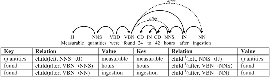
We also found it helpful to have features about the path to the nearest protein, regardless of distance. In cases of multiple shortest paths, we took only one, exploring the dependency tree generally in left to right order. For each potential trigger, we looked at the dependency edge labels leading to that nearest protein. In addition we had a feature including both the dependency edge labels and the token text (lowercased) along that path. Finally, we had a feature indicating whether some token along that path was also in the trigger gazetteer. The formulation of this set of features is still not optimal especially for the “binding” events as the training data will include paths to more than one protein argument. Nevertheless, in Table 3, Key Relation Value Key Relation Value

quantities child(left, NNS՜JJ) measurable measurable child-1(left, NNS՜JJ) quantities found child(after, VBN՜NNS) hours hours child-1(after, VBN՜NNS) found found child(after, VBN՜NN) ingestion ingestion child-1(after, VBN՜NN) found

we can see that this set of features contributed to improved precision.

Cluster Features. Lexical and stem features were crucial for accuracy, but were unfortunately sparse and did not generalize well. To mitigate this, we incorporated word cluster features. In addition to the lexical item and the stem, we added another feature indicating the cluster to which each word belongs. To train clusters, we downloaded all the PubMed abstracts (http://pubmed.gov), parsed them with a simple dependency parser (a reimplementation of McDonald, 2006 trained on the GENIA corpus), and extracted dependency relations to use in clustering: words that occur in similar contexts should fall into the same cluster. An example sentence and the relations that were extracted for distributional similarity computation are presented in Figure 2. We ran a distributional similarity clustering algorithm (Pantel et al., 2009) to group words into clusters.

Tfidf features. This set of features was intended to capture the salience of a term in the medical and “general” domain, with the aim of being able to distinguish domain-specific terms from more ambiguous terms. We calculated the tf.idf score for each term in the set of all PubMed abstracts and did the same for each term in Wikipedia. For each token in the input data, we then produced three features: (i) the tf.idf value of the token in PubMed abstracts, (ii) the tf.idf value of the token in Wikipedia, and (iii) the delta between the two values. Feature values were rounded to the closest integer. We found, however, that adding these features did not improve results.

2.2.2 Feature combination and reduction

We experimented with feature reduction and feature combination within the set of features described here. For feature reduction we tried a number of simple approaches that typically work well in text classification. The latter is similar to the task at hand, in that there is a very large but sparse feature set. We tried two feature reduction methods: a simple count cutoff, and selection of the top n features in terms of log likelihood ratio (Dunning, 1993) with the target values. For a count cutoff, we used cutoffs from 3 to 10, but we failed to observe any consistent gains. Only low cutoffs (3 and occasionally 5) would ever produce any small improvements on the development set. Using

log likelihood ratio (as determined on the training set), we reduced the total number of features to between 10,000 and 75,000. None of these experiments improved results, however. One potential reason for this negative result may be that there were a lot of features in our set that capture the same phenomenon in different ways, i.e. which correlate highly. By retaining a subset of the original feature set using a count cutoff or log likelihood ratio we did not reduce this feature overlap in any way. Alternative feature reduction methods such as Principal Component Analysis, on the other hand, would target the feature overlap directly. For reasons of time we did not experiment with other feature reduction techniques but we believe that there may well be a gain still to be had.

2.3

This phase of the pipeline was again modeled as multi-class classification. There could be an edge originating from any trigger word and ending in any trigger word or protein. Looking at the set of all such edges, we trained a classifier to predict the label of this edge, or NONE if the edge was not present. Here we found that a maximum entropy classifier performed somewhat better than an SVM, so we used an in-house implementation of a maximum entropy trainer to produce the models.

2.3.1 Features for Edge Detection

As with trigger detection, our initial feature set for edge detection was strongly influenced by features that were successful in Björne et al. (2009). Additionally, we included the same dependency path features to the nearest protein that we used for trigger detection, described in 2.2.1. Further, for a prospective edge between two entities, where the entities are either a trigger and a protein, or a trigger and a second trigger, we added a feature that indicates (i) if the second entity is in the path to the nearest protein, (ii) if the head of the second entity is in the path to the nearest protein, (iii) the type of the second entity.

2.4

Given the set of edges, we used a simple deterministic procedure to produce a set of events.

This step is not substantially different from that used in prior systems (Björne et al., 2009).

2.4.1 Balancing Precision and Recall

As in Björne et al. (2009), we found that the trigger detector had quite low recall. Presumably this is due to the severe class imbalance in the training data: less than 5% of the input tokens are triggers. Thus, our classifier had a tendency to overpredict NONE. We tuned a single free parameter ߚ א Թା

(the “recall booster”) to scale back the score associated with the NONE class before selecting the optimal class. The value was tuned for whole-system F-measure; optimal values tended to fall in the range 0.6 to 0.8, indicating that only a small shift toward recall led to the best results.

Development Set Test Set

Event Class Count Recall Precision F1 Count Recall Precision F1

Gene_expression 749 76.37 81.46 78.83 1002 73.95 73.22 73.58 Transcription 158 49.37 73.58 59.09 174 41.95 65.18 51.05 Protein_catabolism 23 69.57 80.00 74.42 15 46.67 87.50 60.87 Phosphorylation 111 73.87 84.54 78.85 185 87.57 81.41 84.37 Localization 67 74.63 75.76 75.19 191 51.31 79.03 62.22

=[SVT-TOTAL]= 1108 72.02 80.51 76.03 1567 68.99 74.03 71.54

Binding 373 47.99 50.85 49.38 491 42.36 40.47 41.39

=[EVT-TOTAL]= 1481 65.97 72.73 69.18 2058 62.63 65.46 64.02

Regulation 292 32.53 47.05 38.62 385 24.42 42.92 31.13 Positive_Regulation 999 38.74 51.67 44.28 1443 37.98 44.92 41.16 Negative_Regulation 471 35.88 54.87 43.39 571 41.51 42.70 42.10

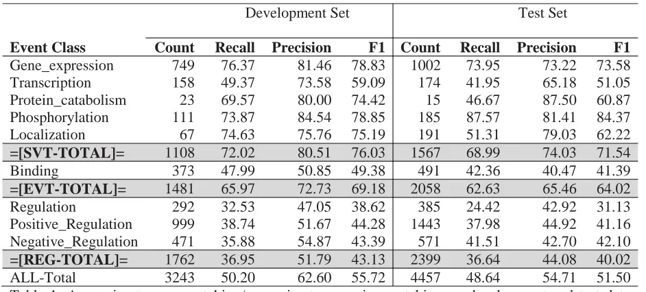
=[REG-TOTAL]= 1762 36.95 51.79 43.13 2399 36.64 44.08 40.02

ALL-Total 3243 50.20 62.60 55.72 4457 48.64 54.71 51.50 Table 1: Approximate span matching/approximate recursive matching on development and test data sets for GENIA Shared Task -1 with our system.

Trigger Detection Features

Trigger

Loss Recall Prec. F1

B 2.14 48.44 64.08 55.18 B + TI 2.14 48.17 62.49 54.40 B + TI + C 2.14 50.32 60.90 55.11 B + TI + C + PI 2.03 50.20 62.60 55.72 B + TI + C + PI

+D

2.02 49.21 62.75 55.16

3

Results

Of the five evaluation tracks in the shared task, we participated in two: the GENIA core task, and the EPI (Epigenetics and Post-translational modifications) task. The systems used in each track were substantially similar; differences are called out below. Rather than building a system customized for a single trigger and event set, our goal was to build a more generalizable framework for event detection.

3.1

Using F-measure performance on the development set as our objective function, we trained the final

system for the GENIA task with all the features described in section 2, but without the conversion rules and without either feature combination or reduction. Furthermore, we trained the cluster features using the full set of PubMed documents (as of January 2011). The results of our final submission are summarized in Table 1. Overall, we saw a substantial degradation in F-measure when moving from the development set to the test set, though this was in line with past experience from our and other systems.

We compared the results for different parsers in Table 3. MCCC-I is not better in isolation but does produce higher F-measures in combination with other parsers. Although posteriors were not particularly helpful on the development set, we ran

Parser

SVT-Total Binding REG-Total All-Total

Recall Prec. F1 Recall Prec. F1 Recall Prec. F1 Recall Prec. F1

MCCC 70.94 82.72 76.38 45.04 55.26 49.63 34.39 51.88 41.37 48.10 64.39 55.07 MCCC-I 68.59 82.59 74.94 42.63 58.67 49.38 32.58 52.76 40.28 46.06 65.50 54.07 Enju 71.66 82.18 76.56 40.75 51.01 45.31 32.24 49.39 39.01 46.69 62.70 53.52 MCCC-I +

Posteriors

70.49 78.87 74.44 47.72 51.59 49.58 35.64 50.40 41.76 48.94 61.47 54.49

MCCC + Enju

71.84 82.04 76.60 44.77 53.02 48.55 34.96 53.15 42.18 48.69 64.59 55.52

MCCC-I + Enju

72.02 80.51 76.03 47.99 50.85 49.38 36.95 51.79 43.13 50.20 62.60 55.72

Table 3: Comparison of Recall/Precision/F1 on the GENIA Task-1 development set using various combinations of parsers: Enju, MCCC (Mc-Closky Charniak), and MCCC-I (Mc-Closky Charniak Improved self-trained biomedical parsing model) with Stanford collapsed dependencies were used for evaluation. Results on Simple, Binding and Regulation and all events are shown.

Development Set Test Set

Event Class Count Recall Precision F1 Count Recall Precision F1

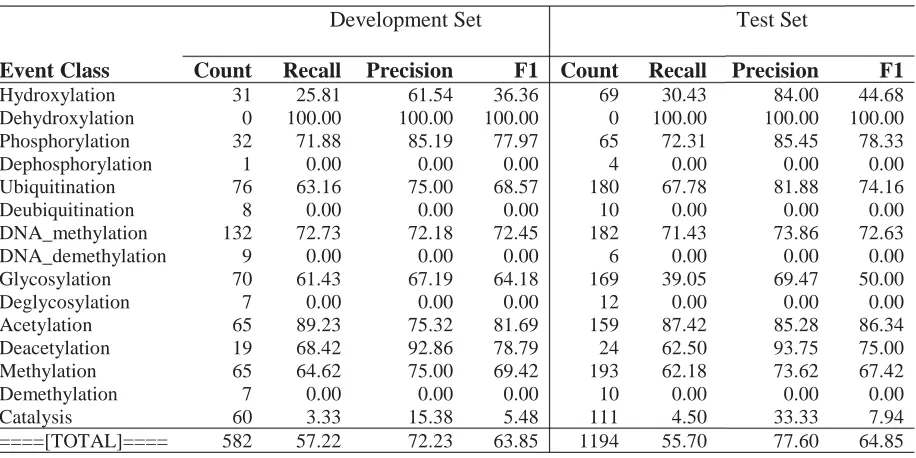
Hydroxylation 31 25.81 61.54 36.36 69 30.43 84.00 44.68 Dehydroxylation 0 100.00 100.00 100.00 0 100.00 100.00 100.00 Phosphorylation 32 71.88 85.19 77.97 65 72.31 85.45 78.33 Dephosphorylation 1 0.00 0.00 0.00 4 0.00 0.00 0.00 Ubiquitination 76 63.16 75.00 68.57 180 67.78 81.88 74.16 Deubiquitination 8 0.00 0.00 0.00 10 0.00 0.00 0.00 DNA_methylation 132 72.73 72.18 72.45 182 71.43 73.86 72.63 DNA_demethylation 9 0.00 0.00 0.00 6 0.00 0.00 0.00 Glycosylation 70 61.43 67.19 64.18 169 39.05 69.47 50.00 Deglycosylation 7 0.00 0.00 0.00 12 0.00 0.00 0.00 Acetylation 65 89.23 75.32 81.69 159 87.42 85.28 86.34 Deacetylation 19 68.42 92.86 78.79 24 62.50 93.75 75.00 Methylation 65 64.62 75.00 69.42 193 62.18 73.62 67.42 Demethylation 7 0.00 0.00 0.00 10 0.00 0.00 0.00 Catalysis 60 3.33 15.38 5.48 111 4.50 33.33 7.94 ====[TOTAL]==== 582 57.22 72.23 63.85 1194 55.70 77.60 64.85

a system consisting of MCCC-I with posteriors (MCCC-I + Posteriors) on the test set after the final results were submitted, and found that it was competitive with our submitted system (MCCC-I + ENJU). We believe that ambiguity preservation has merit, and hope to explore more of this area in the future. Diversity is important: although the ENJU parser alone was not the best, combining it with other parsers led to consistently strong results. Table 2 explores feature ablation: TI appears to degrade performance, but clusters regain that loss. Protein depth information was helpful, but dependency rule conversion was not. Therefore the B+TI+C+PI combination was our final submission on GENIA.

3.2

We trained the final system for the Epigenetics task with all the features described in section 2. Further, we produced the clusters for the Epigenetics task using only the set of GENIA documents provided in the shared task.

In contrast to GENIA, we found that the dependency rule conversions had a positive impact on development set performance. Therefore, we included them in the final system. Otherwise the system was identical to the GENIA task system.

4

Discussion

After two rounds of the BioNLP shared task, in 2009 and 2011, we wonder whether it might be possible to establish an upper-bound on recall and precision. There is considerable diversity among the participating systems, so it would be interesting to consider whether there are some annotations in the development set that cannot be predicted by any of the participating systems1. If this is the case, then those triggers and edges would present an interesting topic for discussion. This might result either in a modification of the annotation protocols, or an opportunity for all systems to learn more.

After a certain amount of feature engineering, we found it difficult to achieve further improvements in F1. Perhaps we need a significant shift in architecture, such as a shift to joint inference (Poon and Vanderwende, 2010). Our system may be limited by the pipeline architecture.

1

Our system output for the 2011development set can be

MWEs (multi-word entities) are a challenge. Better multi-word triggers accuracy may improve system performance. Multi-word proteins often led to incorrect part-of-speech tags and parse trees.

Cursory inspection of the Epigenetics task shows that some domain-specific knowledge would have been beneficial. Our system had significant difficulties with the rare inverse event types, e.g. “demethylation” (e.g., there are 319 examples for “methylation” in the combined training/development set, but only 12 examples for “demethylation”). Each trigger type was treated independently, thus we did not share information between an event and its related inverse event type. Furthermore, our system also failed to identify edges for these rare events. One approach would be to share parameters between types that differ only in a prefix, e.g., “de”. In general, some knowledge about the hierarchy of events may let the learner generalize among related events.

5

Conclusion and Future Work

We have described a system designed for fine-grained information extraction, which we show to be general enough to achieve good performance across different sets of event types and domains. The only domain-specific characteristic is the pre-annotation of proteins as a special class of entities. We formulated some features based on this knowledge, for instance the path to the nearest protein. This would likely have analogues in other domains, given that there is often a special class of target items for any Information Extraction task.

Our immediate plans to improve our system include semi-supervised learning and system combination. We will also continue to explore new levels of linguistic representation to understand where they might provide further benefit. Finally, we plan to explore models of joint inference to overcome the limitations of pipelining and deterministic post-processing.

Acknowledgments

We thank the shared task organizers for providing this interesting task and many resources, the Turku BioNLP group for generously providing their system and intermediate data output, and Patrick Pantel and the MSR NLP group for their help and support.

References

Jari Björne, Juho Heimonen, Filip Ginter, Antti Airola, Tapio Pahikkala and Tapio Salakoski. 2009. Extracting Complex Biological Events with Rich Graph-Based Feature Sets. In Proceedings of the Workshop on BioNLP: Shared Task.

Thomas Cormen, Charles Leiserson, and Ronald Rivest. 2002. Introduction to Algorithms. MIT Press.

Ted Dunning. 1993. Accurate methods for the statistics of surprise and coincidence. Computational Linguistics, 19(1), pp. 61-74.

George E. Heidorn, 2000. Intelligent Writing Assistance. In Handbook of Natural Language Processing, ed. Robert Dale, Hermann Moisl, and Harold Somers. Marcel Dekker Publishers.

Karen Jensen. 1993. PEGASUS: Deriving Argument Structures after Syntax. In Natural Language Processing: the PLNLP approach, ed. Jensen, K., Heidorn, G.E., and Richardson, S.D. Kluwer Academic Publishers.

Marie-Catherine de Marneffe, Bill MacCartney and Christopher D. Manning. 2006. Generating Typed Dependency Parses from Phrase Structure Parses. In

LREC 2006.

Yusuke Miyao and Jun’ichi Tsujii. 2008. Feature forest models for probabilistic HPSG parsing.

Computational Linguistics 34(1): 35-80.

David McClosky and Eugene Charniak. 2008. Self-Training for Biomedical Parsing. In Proceedings of the Association for Computational Linguistics 2008.

David McClosky. 2010. Any Domain Parsing: Automatic Domain Adaptation for Natural Language

Parsing. Ph.D. thesis, Department of Computer Science, Brown University.

Ryan McDonald. 2006. Discriminative training and spanning tree algorithms for dependency parsing. Ph. D. Thesis. University of Pennsylvania.

Haitao Mi, Liang Huang, and Qun Liu. 2008. Forest-based Translation. In Proceedings of ACL 2008, Columbus, OH.

Patrick Pantel, Eric Crestan, Arkady Borkovsky, Ana-Maria Popescu and Vishnu Vyas. 2009. Web-Scale Distributional Similarity and Entity Set Expansion. In

Proceedings of EMNLP 2009.

Hoifung Poon and Lucy Vanderwende. 2010. Joint inference for knowledge extraction from biomedical literature. In Proceedings of NAACL-HLT 2010.

Martin.F. Porter, 1980, An algorithm for suffix stripping, Program, 14(3):130−137.