Prediciton of fatigue failure in engineering components using the finite element method

OUscoil Atha Cliath The University of Dublin

Terms and Conditions of Use of Digitised Theses from Trinity College Library Dublin Copyright statement

All material supplied by Trinity College Library is protected by copyright (under the Copyright and Related Rights Act, 2000 as amended) and other relevant Intellectual Property Rights. By accessing and using a Digitised Thesis from Trinity College Library you acknowledge that all Intellectual Property Rights in any Works supplied are the sole and exclusive property of the copyright and/or other I PR holder. Specific copyright holders may not be explicitly identified. Use of materials from other sources within a thesis should not be construed as a claim over them.

A non-exclusive, non-transferable licence is hereby granted to those using or reproducing, in whole or in part, the material for valid purposes, providing the copyright owners are acknowledged using the normal conventions. Where specific permission to use material is required, this is identified and such permission must be sought from the copyright holder or agency cited.

Liability statement

By using a Digitised Thesis, I accept that Trinity College Dublin bears no legal responsibility for the accuracy, legality or comprehensiveness of materials contained within the thesis, and that Trinity College Dublin accepts no liability for indirect, consequential, or incidental, damages or losses arising from use of the thesis for whatever reason. Information located in a thesis may be subject to specific use constraints, details of which may not be explicitly described. It is the responsibility of potential and actual users to be aware of such constraints and to abide by them. By making use of material from a digitised thesis, you accept these copyright and disclaimer provisions. Where it is brought to the attention of Trinity College Library that there may be a breach of copyright or other restraint, it is the policy to withdraw or take down access to a thesis while the issue is being resolved.

Access Agreement

By using a Digitised Thesis from Trinity College Library you are bound by the following Terms & Conditions. Please read them carefully.

Prediction of Fatigue Failure in

Engineering Components Using the

Finite Element Method

Ge W ang

Submitted in fulfilment of the requirements for the award of the degree of Doctor of

Philosophy to The University of Dublin, Trinity College, October 1999.

Supervisor:

Professor David Taylor

Table o f Contents

...

i

Declaration

...v

Acknowledgements

...

vi

Summary

...

vii

Nomenclature

...

viii

Chapter 1 Introduction.

...

1

Chapter 2 Review o f the Literature

...

3

2.1 Traditional Approaches for Prediction of Fatigue FaUure... 3

2.1.1 Stress life method...3

2.1.2 Strain life method... 4

2.1.3 Critical distance m ethods... 5

2.2 Fracture Mechanics Methods...6

2.2.1 Smith and Miller method... 7

2.2.2 Crack Modelling M ethod... 9

2 3 Consideration of Crack Closure and Defect Effects...11

2.3.1 Newman’s model, considering crack closure...11

2.3.2 Murakami and Endo’s model: considering defects and hardness... 12

2.4 Short Crack Problems... 14

2.4.1 Kitagawa and Takahashi Curve...15

2.4.2 ElHaddad Model; parameter Uo...16

Chapter 3 Further Study o f the Crack Modelling Method.

...

19

3.1 Introduction...19

3 2

The Focus Path---...--- 19

3.2.1 Path orientation, the rule of lowest AKf e

... 19

3.4 Conclusions...39

Chapter 4 Modification o f CMMfor the Short Crack Problem

...

40

4.1 Introduction...40

4.2 Method 1 — Comparing with

Acr^

... 40

4 3 Method 2 —Using a„ as the equivalent crack length...44

4.4 Method 3 — Adding ao or extrapolating the stress/distance curve... 48

4.5 Method 4 - Average of NM & CMM...— ..—...— ...—.— ..—.— ...—..51

4.6 Conclusions... ...

...54

Chapter 5 A New Method o f Prediction

...

56

5.1 Introduction...56

5.2 Background of the Theoretical Model ...56

5 3 New Approach to Find the Critical Distance... 57

5.3.1 Point Method... 59

5.3.2 Line Method... 60

5.3.3 Area Method... 61

5.4 Application o f the Model to Short C racks... 63

5.5 Application of the Model to Notches

...65

5.6 Discussion...66

5.6.1 Input parameters needed... 66

5.6.2 Comparison of the new methods with previous approaches... 66

5.6.3 Extension to other loading modes... 67

5.6.4 Further work...68

5.7 Conclusions...*.—....—... 69

Chapter 6 Notched Specimen Verification

...

70

6.2.1 Steel samples...71

6.2.2 Aluminium alloy samples... 73

6.2.3 Cast iron samples... 74

6 3

Stress Analysis...75

6.3.1 Element type...75

6.3.2 Load condition... 76

6.4 Definition of Prediction Error... 77

6.5 Prediction Results...78

6.5.1 Verification of steel samples... 79

6.5.2 Verification of aluminium alloy samples... 89

6.5.3 Verification of cast iron samples...92

6.5.4 Summary of verification...93

6.6 Discussion...

94

6.7 Conclusions...97

Chapter 7 Prediction o f The Fatigue Failure in Engineering Components...

99

7.1 Marine Component

... 99

7.1.1 Fatigue feilure description... 99

7.1.2 Prediction results from CMM, PM and N M ... 101

7.1.3 Conclusions... 102

7J2 Crankshaft... 102

7.2.1 Introduction... 102

7.2.2 Material and experimental data...103

7.2.3 Prediction result...105

7.2.4 Conclusions...106

7 3 Camshaft...107

7.3.1 Introduction...107

7.3.2 Experimental details... 107

7.3.5 Prediction of fetigue limit...113

7.3.6 Discussion... 116

7.3.7 Conclusions... 117

7.4 Al-alloy Components...118

7.4.1 Introduction...118

7.4.2 Experimental details...118

7.4.3 Results...123

7.4.4 Estimation of threshold

AK.th

... 126

7.4 4.1 Short crack effect...126

7.4.4.2 Procedure... 126

7.4.4.3 Prediction results... 127

7.4.4.4 Kitagawa and Takahashi curves of LM 25...127

7.4.5 Fatigue failure prediction... 128

7.4.5.1 Definition of

(J-r

curve path... 128

7.4.5.2 Prediction results and discussion... 131

7.4.6 Conclusions...133

7.5 General Conclusions for the Application to Engineering Components ... 133

Chapter 8 Discussion, General Methodology and Conclusions

...

135

8.1 Discussion... 135

8.1.1 Overview o f Chapters 6 and 7...135

8.1.2 Critical distance methods... 137

8.1.3 Crack Modelling Method combined with the Notch Method...138

8.2 General Methodology... 139

8 3 Conclusions...143

I declare that the present work has not been submitted as an exercise for a degree at any other

University. This thesis consists entirely of my own work except where references indicate

otherwise.

I would like to thank all those who helped in this research. In particular I would like to thank

and congratulate my supervisor Professor David Taylor, for his guidance, suggestions,

advice, insight and help in creating this thesis. I would also like to thank him for my

involvement in the Rover Group and E)AC Ltd, which were beneficial to my research.

I am very grateful to all the technical staff, Frank, John, Ray, Tom, Gabriel, Gerry and Danny

for all their help and friendship. A special thanks to Peter and Sean who were always willing

to give up their time to help with my research. I am very grateful to Virginia and Joan for

their kind help.

The financial support provided by Materials Ireland, Enterprise Ireland and Rover are

gratefully acknowledged.

I am also very grateful to all the postgraduates and staff at Trinity College, for it was they

who made my stay enjoyable, in particular I would like to thank Conor, Magali, Carlos,

Peter, Damien, Liam, Darren, Gavin, Bruce, Suzanne and Linda. I would especially like to

thank Jeff Badger and Toman MacGinley for their advice, letter writing abilities, computer

skill and their friendship. I would also like to thank Dr. Youhe Zhang for his kind help and

friendship.

I would like to convey my deepest appreciation to my mother and father, my parents in law,

for their continuous support, encouragement, help, advice and patience.

Prediction of fatigue failure in engineering artefacts is becoming increasingly important as

we enter the third millennium; more catastrophic fatigue failures will occur as engineers push

the limits of design even further due to demands for greater efficiency. This thesis describes a

methodology for predicting fetigue feilure in engineering components subjected to high cycle

fatigue using the finite element analysis method.

The research started fi'om a previous theory known as the “crack modelling method” , which

considers the whole stress field and models a geometrical discontinuity as a crack. Further

study of the theory was carried out and improvements were made for application to the short

crack/notch problem. Because of the difficulty o f judging whether a defect in a given

component would behave as a short crack or not in practice, a new approach was developed.

The method was still based on a consideration of the stress field of the component, but

attention was focussed on a small region close to the stress concentration. The method avoids

the problem because it inherently allows for short crack effects. The basic theory was

formulated and tested, with respect to standard test specimens, for which data was found

fi'om the literature. The effect of notch depth, of notch acuity, of notch and specimen type, of

load ratio, and of material properties on the notched fatigue limit were considered. The

theory showed good predictions. The implication of this research is that there is no

fundamental difference between the fatigue limit of an uncracked body and that of a body

which already contains a crack. The theory was also tested on real components used in

vehicles, including a crankshaft, camshaft, pump bracket and C-shaped bracket. Good

predictions were achieved in all cases.

Symbol

'^jarea

a

au <^2

aw

AM

A„

Ave.

C

CMM

CMMscr

CNB

CNP

D

da/dN

DENP

dp

ElHaddad

F

h

Unit

Definition

mm

Murakami defect geometrical parameter

mm

Crack length

mm

ElHaddad crack-length constant

mm

Taylor and Knott crack length related to short crack

mm

Equivalent crack length

mm

Half crack length of a central crack in an infinite plate

Area Method

Constant whose value depends on the strength and ductility of

the material

Average Method

Constant factor in the Paris equation

Crack Modelling Method

Crack Modelling Method with short crack correction

Circumferential notch cylindrical bar

Centre notch in a flat plate

mm

Notch depth

Crack growth rate

Double edge notch in flat plate

Peripheral density factor

Radial density factor

LEFM prediction modified using ElHaddad’s correction

Geometrical factor in the stress intensity equation

Volume fi'action of graphite

mm

Notched specimen height

Hv,gross

Gross Vickers hardness value including the contribution

graphite nodules

K

MPam^'^

Stress intensity factor

K&L

Klesnil and Lucas Method

K f

Fatigue notch factor

K ,

Theoretical elastic stress concentration fector

k:

Critical value of

Kt

Ke

Strain concentration factor

Ka

Stress concentration factor

L

mm

Notched specimen length

I

mm

Effective length of plain specimen

LEFM

Standard crack prediction method following Smith and Mil

when applied to notches

LM

Line Method

h

mm

Average element length round a fillet or a notch root

mm

Average element length along the radial direction

n

Empirical exponent in the Paris equation

N f

Fatigue cycles to failure

NM

Notch Method

PM

Point Method

r

mm

Distance from notch/crack tip or stress concentration

R

Load ratio

fmint ^m ax

mm

Minimum and maximum distance of a stress-distance curve

SENP

Single edge notch in flat plate

W

mm

Notched specimen thickness

AFy

N

Axial input force applied to a finite element model

MPam^^

Range of the stress intensity factor

A Kfe

M Pam '^

Predicted threshold stress intensity factor range using FEA

MPa m '^

Threshold stress intensity factor range

APo

Predicted fatigue limit load range

A Pt

Experimental value of fatigue limit range

Act

MPa

Stress range

AcTo

MPa

Fatigue limit of plain specimens

A Goc

MPa

Fatigue limit of cracked specimens (nominal stress)

^^on

MPa

Fatigue limit of notched specimens (nominal stress)

ACTPRED

MPa

Predicted fetigue limit

AcTth

MPa

Threshold stress range

Act gross

MPa

Fatigue limit in gross-section

T

mm

Plain specimen thickness

a ,p

Degrees

Angle of the path of a stress-distance curve

X

mm

Distance measured from centre of a hole

5

mm

Distance between the axis and the point where

is applied

<

!>

mm

Specimen diameter

Correcting factor for short crack effect

P

mm

Notch root radius

*

P

mm

Critical value of

CT

MPa

Stress

CTcy

MPa

Cyclic yield stress

CT-r

Stress-distance curve

Ow

MPa

Tensile stress applied to an infinite plate in Westergaard’s

equation

Fatigue is the most common cause of failure of engineering structures and components.

Making reliable fatigue predictions is very difficult because knowledge about fatigue

mechanisms in all stages of the fatigue process must be developed much further. Despite the

huge volume of research which has been conducted in this area and many hundreds of papers

and reports published each year on the problem of fatigue life prediction, it remains the

principal limitation on the life prediction of components, especially components such as

aircraft, vehicles, medical devices and machine tools.

The aim of the present research has been to develop methods of analysis for the prediction of

the high cycle fatigue (HCF) behaviour in engineering components using the finite element

analysis (FEA) method. Traditional methods, which compute fatigue life on a point-by-point

basis, could not give a satisfied prediction when applied to high stress concentrations (e.g.

sharp notches) or to materials of low notch-sensitivity (e.g. cast iron). The reason is that very

high stresses can be tolerated by a component provided they are restricted to small regions of

the component and then there is no one to one relationship between stress and life.

The crack modelling method developed by Taylor [1996], which considers the whole stress

field and models the geometrical feature, such as a notch, a hole and a corner, as a crack, was

tried in this thesis. Further study was done on the method, such as the path determination, the

minimum and maximum distance. With these improvements the method was tested using

some simple specimens from the literature and in-house. The method was also tested on a

real engineering component which was used by Rover car company. The results were very

promising in many cases.

materials such as cast irons, cast aluminium alloys. Several attempts were tried to modify the

method in order to overcome the difficulties. These included adding a material constant,

adding a short crack length in a notched body and combining the method with a traditional

stress-life method. Different modifications were made for different situations and the revised

method was tested on notched specimens showing short crack effect. The prediction results

on the simple geometrical specimens showed a good agreement with the experimental data.

However, a problem arose when feced with real engineering components with complex

geometry. The difficulty was how to know whether a given geometrical feature would be a

short crack problem or not. We went back to basics and made big modifications to the

previous theory. The new theory was devised based on a consideration o f the stress field of

the component, but now attention was focussed on a small region close to the stress

concentration. Three methods were formulated: the point method, the line method and the

area method. Each of them has its own advantage. They inherently allowed for the short

crack effect, so they should avoid the problem found in the previous approach theoretically.

Ten methods including traditional stress-life methods, the crack modelling method and its

revised versions and the new methods were tested on standard test specimens, for which data

can be found from the literature. The effect of notch depth, of notch acuity, of notch and

specimen type, of load ratio, and of material properties on the threshold stresses were

considered. The theory showed good predictions on 90 percent of forty-six data sets.

Furthermore, four types of real components were used for testing thanks to Rover Car

Company and GEC Ltd. Some of the components had surfece effects and for some of them

we needed to measure the fatigue threshold. All these difficulties were overcome and good

results were obtained, showing that the new methods can be applied to real components.

Engineering structures invariably contain stress concentrations which are the principal sites

for the inception of fatigue flaws. The stress and deformation fields in the immediate vicinity

of the stress concentration have a strong bearing on how the fetigue cracks nucleate and

propagate. Continuum approaches on this topic can be divided into four categories. They are

traditional approaches (which include stress-life, strain-life and critical distances), fracture

mechanics concepts, crack closure & defect effects and the short crack problem.

The effect of stress concentrators on fetigue limit and high-cycle endurance has traditionally

been studied using notches. The simplest approach - using the elastic stress-concentration

fector

Kt

- is reasonably accurate for blunt notches under low applied stress, but ATt is found

to diverge from the experimentally measured fatigue strength reduction,

Ki,

when notches are

sharp or when the notch depth,

D,

is small. Relevant factors include the existence of the

plastic zone and the relatively small stressed volume ahead of a sharp notch.

2.1 Traditional Approaches for Prediction of Fatigue Failure

2.1.1 Stress life method

The stress-life approach is used for high-cycle fatigue failures ahead of stress concentrations.

High cycle fatigue (HCF) is caused by low, nominally elastic fluctuating stresses. The

prediction of fatigue failure is made by appropriately modifying the smooth specimen

(unnotched) endurance limit.

(2-

1-

1)

where

p

is the radius at the ends of the ellipse and

D

is the depth (half width) of the elliptical

hole.

The stress-life method is unsuitable for situations where considerable plastic deformation

occurs ahead of the stress concentration.

2.1 .2 Strain life m ethod

The local strain approach relates deformation occurring in the immediate vicinity of a stress

concentration to the remote stresses and strains using the constitutive response determined

from fetigue tests on simple laboratory specimens. The method predicts the life expectancy

of a machine part which is under low cycle fatigue loads. Low cycle fatigue (LCF) is caused

by high, fluctuating stresses and strains. The method has its beginning in the early 1950s.

Today it is still in frequent use by machine designers in LCF and HCF analyses and it is

recommended by ASME [ASME, 1989], SAE [Rice, 1988] and ASTM [ASTM, 1980].

The strain concentration factor

is the ratio of the maximum local strain to the nominal

strain. The stress and strain concentration factors are of the same value when only elastic

deformation occurs at the tip of the notch. However, once the material yields at the notch tip,

the stress and strain concentration factors take different values. Under conditions of plastic

deformation, the theoretical elastic stress concentration factor is given approximately by the

geometrical mean of the stress ATcrand strain concentration factors

K^.

This is the well-known

Neuberrule [Neuber, 1961]:

First, the local stress and strain histories at the notch tip must be known. Second, the fetigue

life that can be expected for the local stress and strain histories must be determined. For the

first part, either simple analytical expressions or detailed finite element simulations o f the

notch tip deformation (using constitutive laws and hardening rules) are developed to relate

the local stresses and strains to far-field loading. Alternatively, the notch tip deformation is

experimentally monitored with the aid of strain gauges or other displacement/strain

measurement techniques.

2.1.3 Critical distance methods

Under fatigue loading conditions, the elastic stress concentration factor is replaced by the so-

called fatigue notch factor;

Kf = unnotched bar endurance limit / notched bar endurance limit

(2-1 -3)

The Peterson equation for ferrous wrought alloys has the form

(2-1-4)

... where

is a constant whose value depends on the strength and ductility of the material

and p

is the notch-root radius. By considering the threshold condition for a crack of length oo

at the notch root, Klesnil and Lucas [1980] derived an equation as follows;

where

is the EHaddad crack-length constant (see Section 2.4.2).

2.2 Fracture Mechanics Methods

The most successful application of the theory of fracture mechanics is in the characterisation

of fatigue crack propagation. One of the known methods is the method of linear elastic

fracture mechanics (LEFM). It is designated to compute the crack propagation based on the

fiindamental assumption that the material is linearly elastic. This method basically

approaches the crack propagation problems in 2-D space. For more complex cases an

adaptation of the basic correlations is used. A very important parameter, called the stress

intensity factor (SIF), was introduced, which signifies the relationship of three factors; the

geometry of the plate, the loading, and the length of the crack. The stress intensity factor is

defined as follows

In the above, F is a compliance function that describes the geometry of the part, cris a stress

in a remote distance which designates the loading and a is the crack length. The crack growth

can be expressed in the form of

^ \ + 4 . 5 a J p

(2-1-5)

—

^C{ AKy

(

2

2

2

where C is a constant factor,

AK

is the range o f the stress intensity factor and

n

an empirical

exponent. The equation is known as the fatigue crack propagation law [Paris and Endoyan,

1963], Crack propagation ceases if

AK < AKth,

the threshold value, which depends on the

load ratio, i? [Taylor, 1989]

2.2 .1 Sm ith and Miller m eth od

Smith and M illers model [Smith and Miller, 1978] can be used for the prediction o f fatigue

failure on notched specimens including the prediction o f non-propagating cracks. It is

illustrated in Fig. 2.2.1, concerning notches with variable radius and constant depth

D.

We

called it the Notch M ethod (NM). For low

Kt

(between A and B) the fetigue limit is given by

where Aoo is the fetigue limit o f plain specimens and Aaon is the fetigue limit o f notched

specimens. For high

Kt

(between B and C) the notch is assumed to behave like a crack, so

the fatigue limit is given by

(2-2-3)

(2-2-4)

X Typical experimental resiills H - - - '

Failure zone

b <

B '

1.0

Stress concentration &ctnr

Fig. 2.2.1 The boundary conditions between failure and non-failure of variously notched

specimens

This model gives good predictions for many materials such as mild steels and alloy steels

[Taylor, 1994] in laboratory tests.

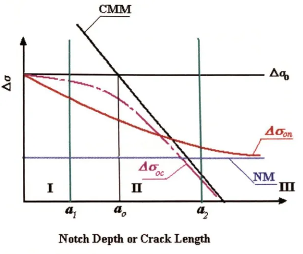
The curve will move up or down in the figure if the notch depth decreases or increases for a

component. So there is not a fixed critical value for the varying notch depths. However there

will be a critical value of the fector,

K*t,

existing at point B in the figure for a certain notch

depth,

D.

At that point, both Eqs. (2-2-3) and (2-2-4) should give the same predictions. So the

critical value can be determined by

(2-2-5)

So for elliptical notches, for example;

AoF-yJnD

where p* is a critical value of the notch tip ratio for the given D. Eq. (2-2-6) deals not only

with the material properties (fatigue limit and material threshold) but also with geometry

characteristics.

The value of

p* can be defined directly using Eq. (2-2-6), if the material properties, such as

fatigue limit and material threshold, are known. This is quite useful for engineering design.

Normally Eqs. (2-2-3) and (2-2-4) are both conservative so they can be used simultaneously

at the point B in Fig.2.2.1.

A problem that remains is that this method could not be directly employed for components

that do not contain notches, but instead have comers or other geometric features where the

stress concentration occurs. This is because neither D nor F

can be defined in these cases.

This greatly reduces the use of this method in engineering applications.

2.2.2 Crack Modelling Method

The crack modelling method [Taylor, 1996] is an extension of the Smith and Miller model.

This extension made the model available for the prediction of engineering components not

only with notches but also with other geometric features.

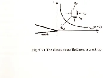
The method examines the stress field in the region of the stress concentration, and compares

this with the stress field that is knovm to exist around an ideal crack. Figure 2.2.2 describes

the approach schematically. From an FE model of the component, loaded with some system

of loads, L, a plot is obtained of stress as a function of distance, r, measured fi'om the point of

maximum stress. The curve in the plot was named as the Stress-Distance curve or

a-r curve

for short. The curve is compared with the stress-distance plot from an ideal crack; the

particular crack geometry chosen is the one examined by Westergaard [1939]: a central,

through crack of length

2a^, in an infinite plate subjected to a tensile stress Ow. This stress

field is described by

The values of

cr„

and

can be varied to obtain a best fit between the stress-distance curve

of Eq. (2-2-7) and the curve obtained from FE data. When the best fit has been found, the

appropriate

K

value is given by

K = (

2

2

8

This method assumes that if the equivalent

AK

is less than the threshold value of the material,

at the appropriate

R

ratio, fetigue feilure will not occur.

lifiiSiMIII

Component FEA

H

Applied Loads, L

Stress

^Ikid^Iioads.L

X‘

r

X

Stresses along X-X' (S-D curve)

Centre-Cracked Infinite Plate

Stress

Stress Inteosit;, K

Stresses along Y-Y*

Best ft ^ves a K prediction

correspondiogto loads L

Fig. 2.2.2 Schematic illustration of the methodology used in the crack modelling

technique

2.3 Consideration of Crack Closure and De^ct Effects

2.3.1 Newman’s model, considering crack closure

Fatigue crack closure is understood to play an important role in many aspects of fetigue crack

growth (FCG) [Elber, 1968], Although closure is not equally important in all FCG problems,

and although closure does not provide a complete explanation of every problem where it is

important, the closure phenomenon is an intrinsic feature of crack tip behaviour that must be

The earliest investigations of closure based on the finite element method were published

independently fi-om 1973 to 1977. One of them is Newman’s model [Newman, 1974; 1981;

1982; 1994], which is called a plasticity-induced crack-closure model. He believed that

crack-closure effects are also one of the key elements in small-crack growth. His model is

based on Elber’s crack-closure phenomenon [Elber, 1970] and the Dugdal model [Dugdale,

I960], Crack-opening stresses were calculated in the model. The J-integral [Rice, 1968], one

of the commonly used parameters for non-linear crack-growth analyses, was used to define

an equivalent plastic stress intensity factor in the elastic-plastic firacture mechanics regime.

The model agreed well with test data on unnotched and notched specimens made of two

aluminium alloys [Wu and Newman, 1993].

Many real closure problems are 3-D, but the computational expense of FE closure analysis

has limited most previous investigations to 2-D. Chermhimi et al. [1988; 1989] performed

the first 3-D FE closure analysis, studying closure through the thickness of a centre-cracked

plate, and more recently publishing some very elementary results for a semi-elliptical surface

crack [Chermhimi et al., 1993]. They generally found higher opening levels at the specimen

surface, similar to plane stress behaviour, and lower opening levels in the specimen interior,

similar to plane strain behaviour. As computational power continues to increase, 3-D FE

closure analysis should become more practical, and many important problems are waiting to

be solved. However, careful study of 3-D modelling issues will be required before the results

can be fiilly trusted.

2.3.2 Murakami and Endo’s model: considering defects and hardness

Murakami and Endo [1983] proposed a model, which considered the defect effect, by

introducing a new geometrical parameter

^jarea for two-dimensional and three-dimensional

defects. This parameter is based on both microscopic observation of cracking fi-om small

surface defects and 3-D numerical stress analysis. From their experiences, they derived the

projecting a defect or a crack onto the plane perpendicular to the maximum tensile stress, n

and c are constants that have to be determined through fatigue tests.

The choice of

^jarea comes from stress intensity factor considerations. Its application has

been widespread, not only to the fatigue problems of small cracks and holes, but also to those

of surfece scratches and roughness, non-metallic inclusions, corrosion-pits, carbides in tool

steels, second phases in Al-Si eutectic alloys and spheroidal graphites in cast irons.

Murakami and colleagues [Murakami

et ah, 1990] further revised the model and proposed

the following equations:

Act^ = 1.4 3 (//,+ 1 2 0 )(> /W a )'^ * (2 - 3 -1 )

AA:^ = 3.3*10-'(//,+120)(V^)''’

(2-3-2)

Here

is the Vickers micro-hardness;

AKth = threshold stress intensity fector range under

the stress ratio R = -I (MPa m’”^);

^area is in

fxm. The extended equation to predict the

fetigue limit for various values of stress ratio R is expressed by including a fector,

in Eq. (2-3-1), where a = 0.226 + //v x 10"^. In predicting

Aoy, by using Eq. (2-3-1), no

fatigue test is necessary. It is sufficient to measure the values of

-\larea and

Hy and to

estimate R at the place where the defect exists. They reported that the prediction error was

less than 15% for //v = 100-740.

In 1991, Endo [1991] proposed a modified equation of this method for nodular cast iron.

Instead of introducing a parameter C, he used the matrix hardness and the percentage of

graphite to predict the fatigue limit ^cr^and AIQh-

This method therefore unifies both effects

of defects and matrix structures:

where //v,

gross

is the gross Vickers hardness value including the contribution o f graphite

nodules and fv is the volume fraction o f graphite. On the other hand,

AKth

is defined as

follows:

^K^=3.3*\0-^

+

(2-3-4)

Murakami and E ndo’s model is valid over a

sjarea

range which is dependent on the

material. The valid upper limit of

^a re a

is considered to be ~ 1000 nm. [Murakami and

Endo, 1994],

2.4

Short Crack Problem s

The fatigue life o f a structure goes through several stages from crack initiation, through crack

propagation, to the final failure. M iller [1993] indicated three categories o f crack growth

regimes for the whole period. They are the micro-structural fracture mechanics (MFM)

regime, the elastic-plastic fracture mechanics (EPFM) regime and the linear elastic fracture

mechanics (LEFM) regime. In the M FM and EPFM regimes, cracks are short and require a

high stress range to propagate. Suresh and Ritchie [1984] suggested the following definitions

by which short cracks can be broadly classified; microstructurally small, mechanically small,

physically small and chemically small cracks. “Small cracks” and “short cracks” are often

used interchangeably. However there is sometimes a distinction between the two cases. The

former definition is employed for flaws that are small in all three dimensions. The latter types

are taken to denote through-thickness flaws that are small in all but one dimension.

Over the past decade, the propagation of short cracks in fatigue has received considerable

attention. The behaviour of short fatigue cracks was reviewed in three books [Miller and de

los Rios, 1986; Ritchie and Lankford, 1986; Suresh, 1991]. Quantitative attempts have been

used to try to explain the propagation and have achieved some success in the correction of

the propagation behaviour.

2.4.1 Kitagawa and Takahashi Curve

Kitagawa and Takahashi [1976] presented a figure similar to Fig. 2.3.1, which shows the

boundary between propagating and non-propagating cracks.

AK. = Y A a (* a )* '^ O

LEFM or loi»g crack-low

.stiess re^ n e

physically small cracks short cracks

shoit crack resiine

lo g

Crack Leii;^h a

Fig.2.3.1. Schematic of the Kitagawa-Takahashi curve showing the boundary between

propagating and non-propagating cracks

less than AKth, but it should also be appreciated that cracks have been reported as growing on

surfaces o f plain specimens at stress levels below the fatigue limit. However, such cracks

eventually stop propagating. This has made some people modify the curve in the

microstructurally short region.

Several other lines can be drawn on the plot, i.e., d\^ (J2, d^, etc., to represent the size of

microstructural units such as grain sizes, inclusion spacing, precipitation spacing, surface

finish, etc., and these too w ill be expected to affect crack growth behaviour. The lengths at

which the experimental data points merge with the plain specimen lim it and the long-crack

threshold were defined by Taylor and Knott [1981] as a \ and uj, respectively. The so-called

the short crack problem is concemed with any crack length that is within a \ and az.

But at crack lengths beyond microstructural effects, i.e., a >«2, it is to be expected that a

continuum mechanics approach w ill represent crack growth behaviour. However, LE FM

analyses o f crack tip fields may not be o f sufficient accuracy at these stresse levels to

describe fatigue crack growth behaviour permitting correspondence between large structures

and small laboratory specimens.

Therefore, fatigue cracks fall into three categories:

(1) microstructurally short cracks: a < oi;

(2) long cracks sometimes termed as LEFM -type cracks: a>az;

(3) transition length cracks: a \ < a < 0 2.

The first category o f short cracks require high stresses for continuous propagation to failure,

i.e., A < j> Acto. The second category is essentially for cracks in low elastic stress fields. The

third category is essentially the short-crack category.

2.4.2

EIHaddad Model: parameter ao

ElHaddad et a l proposed a method for dealing with the short crack problem [EIHaddad et a l ,

which the elastic stress intensity factor (SIF) of a crack is modified by giving it an effective

length of

(a+ao)

AK =

A(TyJn:{a + a^)

(2-4-1)

where

is the applied nominal stress range, and a o

is a constant for a given material and

heat treatment. Actually it was Smith [1977] who first introduced the concept of the

parameter

Oo

and named it as intrinsic crack length. The threshold stress at a very short crack

length will approach the fatigue limit of the material

('AcTo),

based on small smooth

specimens, and from Eq. (2-4-1) the threshold stress intensity

AKt/,

can be obtained as

These equations assume a geometry fector,

F,

equal to unity. Following this model, for any

crack of length a, the threshold stress Aath is then obtained as.

This relationship was tested with a series of experiments on steel and aluminium alloys by

the authors. Short cracks were initiated at notches in these experiments and then they

machined away the notches and determined the threshold stress levels for the cracks. Because

cracks fi-equently start from notches, brittle materials that often break due to crack growth

were sometimes referred to as notch sensitive. As stated in their papers, agreement of the

(2-4-2)

or

a.O

(2-4-3)

prediction of the model (Eq. (2-4-4)) and the test data were very good. Taylor and O ’Donnell

[1994] also tested this theory and found it to apply to a wide range of materials.

For many materials such as mild steels, alloy steels and other alloys, the values of

Oo

are very

small [Ting and Lawrence, 1993] and can be neglected compared with notch depth. For

example, A533B Steel,

ao=0.0762

mm; AISI4340 Steel,

ao=0.0508

mm; AL2024-T351 Alloy

[DuQuesnay

et al, 1986], Oo =0.1016 mm. Therefore, when

K ^ K ^ , the sharp notched

specimens are ‘crack-like’, and Smith and Miller’s model is quite efficient for predicting the

fatigue failure. However, the correlation with experimental data was found to be very poor

when Smith and Miller s model was used to test for the data o f some other materials, like cast

iron. Taylor and colleagues [Taylor

et al, 1996] solved this problem by introducing a

material constant, Uc. The notch depth is augmented by it, thus modelling the notch as a crack

of length (D+ ac). It was shown that the value of Oo is similar to the short crack parameter Oo.

In ElHaddad s model the physical meaning of

a„

is unclear. However it is a reasonable

approximation. And the addition of the geometry factor, F, which contains Oo, to Eq. (2-2-8),

may be better for getting a material constant, ao. Combinations of Smith s model and

ElHaddad s model could be used for prediction of fatigue failure in notched specimens or

Method

3.1 Introduction

The research in this thesis started from the crack modelling method (CMM). The previous

work made by Taylor and his colleagues [Taylor and Lawless, 1996] had showed its success

in 2-D problems and potential advantages in application on engineering components. Further

work needed to be carried out in order to make the technique more suitable for a wide range

of applications for both scientific and engineering usage. This work included the study o f the

path distance effect, the mesh density effect, and the path orientation effect. In this chapter,

all these effects will be examined.

3.2 The Focus Path

The prerequisite for the application o f CMM is that the geometric feature o f a specimen or

component has some features of a real crack, such as a

singularity. The method

examines the stress field in the region o f this feature. Furthermore only one path on which a

stress-distance (o=-r) curve is determined in this region is needed for evaluating the stress

intensity from the FEA,

This specific path is defined as the “ focus path”. Although

previous work had shown some characteristics o f the focus path, it is still worth discussing

how to choose this path, in order to develop a systematic way of choosing this path which

will be used throughout this work.

3.2.1 Path orientation, the mle of lowest A Kf e

The path for CMM is a straight line which radiates from the stress concentration point.

Assuming that a fatigue crack is loaded in M ode I, where the crack’s sides move

perpendicularly apart, the opening stress, i.e. the maximum principal stress (MPS), will drive

the crack to grow. So the path direction should represent the direction on which the crack will

direction [Taylor

et a l,

1997], In that case, the direction of crack growth could be understood

by examining a failed component. The prediction agreed well with the experimental data usin

the path direction. Also if the MPS direction is perpendicular to the crack front, the path

direction should be normal to the MPS direction. It is true that the MPS direction will change

during the crack propagation. Keeping the path normal to the MPS direction from the

beginning to the end will be very difficult, and in doing so the path will be a curve instead of

a straight line. However, we will not make the path like this. We concentrate on the total life

of a component or specimen, in which crack initiation and early growth takes the most part.

We assume that the MPS is the main driving force for fatigue failure. So the MPS direction

here only refers to the MPS direction at or near to the stress concentration place.

Experimental testing was carried out on a single-edge notched specimen, which was

subjected to pull-push loads; the notch depth was 3 mm; the material of the specimen was a

cast Al-alloy, LM25; the fetigue limit o f plain specimens

ACo

was 77.48MPa; the threshold

AKth

was 5.97 MPa m*^^ [Wang

et a l,

1999]. The stress field was analysed using the finite

element method. Fig. 3.2.2 shows MPS contour plot of the specimen. In this case,

which is

defined in Fig. 3.2.1, is equal to zero. Examining a foiled specimen, a crack surface was at a

symmetrical plane a = 0, as shown in Fig.3.2.1. So the path should be at a = 0. A series of

lines are drawn with variable

values for comparison. Fig. 3.2.3 shows the

curves at

variable a values. Fig.3.2.4 shows the effect of the path orientation on value of

using

applied load equal to the experimental fatigue limit.

At or = 0, the prediction error is only 7.03%. It is evident that our assumption is right.

Moreover, the value of

varied from 0° to 60° without any large change in

and even at

60°

the change in

AK/^

was only 15%. This illustrates that the CMM is not sensitive to the

path direction. This character is very good for applications.

Fig. 3.2.1 Path choice on a 3D model of a single-edge notched specimen

140

a = 0 120

0) 100

80 a = 60

60

40

10

0 2 4 6 8

D istance r mm

Fig. 3.2.3

Aa^r

curves of the single notched specimen

S

_u

U.

£ E

4- ■

Measured stress intensity

Threshold value

(0

tf)

b

CO 2 ■ ■

80 60

40 20

0

Angle a

Fig.3.2.4 Path direction eflfect on predicted result using CMM

theoretically; if the value of

AKfe

from the path is more than the threshold value, feilure will

occur. For the above example, the path is at or = 0, which is normal to the MPS direction.

How does this path differ from the others?

2D Stress Fields

The

« = 0°, 3 0° and 60°, are shown. A distinguishable difference can be seen. Starting from an

identical point, the hot spot, each curve has the same maximum stress value; ending at points

where stress field tends to be uniform, the curves tend to be overlapped after a distance. The

difference among each line is that the rates of the stress reduction with increasing

different. Increasing

a

reduces the rate of reduction; the highest rate is at a = 0. All these

result in variable

AK^e

values when using CMM. The variation in a certain region is

monotonic; a curve with a higher rate brings a lower

AKe^

value. On the path a = 0, the

stress in the

curve decreases fester than from a path drawn at any other angle, as

shown in the figure. This results in the lowest value o f

AKfe

from any other path. We call this

phenomenon the “Rule of lowest

AKfe'.

For a component with a complex geometry, a set of stress/distance curves would be drawn

from the stress concentration point and the CMM could give a

AKpe

value on each curve.

However, only one from the path that is normal to the MPS direction is the right answer. The

rule of lowest

AKfe

can be used to identify the MPS direction and give the solution at the

same time.

3D Stress Fields

hi order to test the rule being available in a 3D stress field, two examples are shown below.

The first example is a 3D model of the single-edge notched bar shown in Fig. 3 .2.1. The size

of the bar is 12x18x140 mm. A tensile stress of 60 MPa is applied to the end of the bar. The

stress concentration place is located at the point F which can be seen if the figure, actually on

contour plot. Fig.3.2.5 shows the evaluation o f

values using CMM on variable lines.

The path o f or = 0 and

produces the lowest

as expected. It proves that the Rule o f

lowest

is right in this case. Also the results show that the diflference on each path is

small.

In a general 3D case where the crack path is not known, the path choice can be divided into

two steps; the first step is drawing a plane which is normal to the MPS direction; the second

step is drawing a series o f lines in this plane, radiating fi-om the hot-spot, and then selecting

the line on which the A K f e

value is found to be lowest. Fig. 3.2.6 shows the detail o f the path

choice. The body is subjected to a load P; the hot spot is at

F; n-n’

is the plane normal to the

MPS direction.

CM

(0 Q .

12

10

8

6

4

40

30

20

10

0

Angle p

y77777777777

Stress contours

Fig. 3 .2.6 Schematic illustration o f choosing the path

The second example is a notched bar subjected to a torsion load (actually an automotive

camshaft). The details o f the fatigue test and the finite element analysis will be shown in

Section 7.3. Fig. 3.2.7 shows the schematic illustration o f the path choice in this situation.

Considering a brittle material bar, such as a cast iron, subjected to torsion, M, the crack

plane,

n-n,

is 45” from an axis o f the bar. This plane is normal to the MPS direction

according to stress analysis. Assuming the fatigue failure starts from a point

the stress

condition at the point is illustrated in the figure; a series o f lines are drawn radiating from this

point; then the

values are evaluated using CMM. It is expected that the path o f

0"

will give the lowest

value. On the camshaft, the same process was carried out. The

evaluating

values on each line are shown in Fig. 3.2.8. Because a notch existed, the

path which gives the lower

value is not

0°; it is about at /? = 15°. However the

difiference in

between the two lines is very small, only 3.7%, Even at /? = 45°, the

difference is still only 9.1%. This proves again that CMM is not sensitive to the path

n-n

<F.,

c

\ \ v

F

Fig. 3.2.7 Schematic illustration of the path choice in a bar subjected a torsion load,

assuming a stress concentration at

F.

18

17.5

17

16.5

16

50

40

30

Fig. 3 .2.8 Evaluating

AKfe

values on variable lines for the camshaft

3.2.2 Minimum distance

For any

Aa-r

curve, the focus path is that part of the curve to be examined, which will be

limited by the minimum distance

r„,i„

and maximum distance

rmax,

shown in Fig. 3.2.9.

Westergaard equation and a

Acr-r

curve from the path mentioned above. The fit error, defined

as the percentage difference between the area under the crack curve and the area under the

Ac-r

curve, is minimised. Eq. (2-2-6) gives a stress value of infinity at r = 0, whereas the FE

data gives a finite stress at this point. If

were zero, the fit error would be infinite. This

implies that the comparison of curves must begin at some value,

rmm,

shown in Fig. 3.2.9.

Theoretically,

rmm

should be as small as possible, but avoid being zero. Numerically, it is

impossible due to the limit of the FE mesh density. Three examples will now be highlighted,

which show the effect of

on different materials, geometry and loads.

Westergaard function

A o-r curve of a component

<

r

r

Fig. 3.2.9 Definition of the minimum distance and maximum distance

The first example is a single-edge notched specimen, as shown in the last section. The

previous work suggested using r„,„ =

Oo

[Taylor, 1996]. The underlying logic of this was that

short fatigue cracks would initiate from the notch at an early stage. These cracks would

typically grow to a length «« and would disrupt the stress field over this distance. In this case,

Oo

is 1.89 mm and the error of the prediction is only 3%, as shown in Fig. 3 .2.10. This result

bring much difference on the prediction for a constant w of 17 mm. Compared with

the biggest difference is less than 17%. It implies that CMM is not sensitive to the choice of

rmin,

at least in this case.

Tension

u

c

^

^ i

(0 (0

£

♦ -I (0

8

6

4

Threshold

2

0

5

3

4

1

2

r mln

mm

Fig. 3.2.10 Effect o f o n the prediction ofLM25 specimen subjected to tension load,

f max

1 "7 mm

ao

= 0.05 mm. Fig. 3.2.11 shows the r„,„ efifect on the evaluation

with a constant

o f 5.05 mm. This data will be used in a later chapter.

Bending

u

(B

U - M

^

f

2 I

® I?

</) t f >

0>

(0

8

6

4

A K FE

2

0

3

1

2

0

r

mm

Fig. 3.2.11 Effect o f

on the prediction of a mild steel specimen subjected to bending,

= 5.05 mm

The third example is the camshaft subjected to torsion loads, as mentioned in the last

section. The material constant

o f this cast iron is 2.24 mm. Fig. 3.2.12 shows the

variation o f

when increasing rm,„. The

value is kept as a constant, 11.25 mm.

Again a good prediction is obtained when

Starting at 0.093 mm, the valid

region for

extends to approx 3.5 mm. In this region the error from any

is less

Torsion

2

18

Threshold

^ ^ ■ ■ I

0

2

4

6

8

rmin

mm

Fig. 3.2.12 Effect of

rmm

on the prediction of a camshaft subjected to torsion load,

11.25 mm

In general, these three examples include three kinds of materials, three kinds of geometries

from the previous examples, all indicate a common trend, i.e. CMM is not sensitive to the

choice of rmm. The conclusion supports Taylor’s suggestion. Furthermore, any selection of 0

<

r„i„

^ «o is valid in all these situations.

3.2.2 Maximum distance

include all information about the stress concentration, i.e. the part over which the geometrical

feature raises stresses above their nominal values. However, in the general case of complex

component geometry, it may not be clear what these nominal stress values are. With this in

mind, a series of

r^ax

values was analysed on a

cr-r

curve in order to find a general rule.

Fig. 3.2.13 shows three typical Acr-r curves; (a) is a common curve firom a stress

concentration in a tensile stress field, such as a single notch plate subjected to tensile stress;

(b) represents a curve from more than two stress concentrations in a body; (c) behaves as a

body subjected to bending; the stress goes negative beyond a neutral axis.

and three kinds of load conditions. They cover a wide range o f applications. The conclusions

According the analysis above and the previous work, it was decided to use the entire tensile

stress distribution for (a) and (c). For (b), it is necessary to examine the curve; the focus part

should be in the region where the <T-r curve is consistently decreasing; several values should

be tested if possible; the final rmax value should give the lowest K

value. The three examples

are still used to verify the decision above. We did not have an example for (b) at this stage, so

this was not considered.

Fig. 3.2.14 shows the predicted

AK

values of the first example, the LM25 single-edge

notched specimen. AK

almost remains a constant on variable Kmax

from 1 mm to 17 mm; the

fit error also keeps about the same level, between 7 and 11 %; the biggest prediction error

comparing with the test data is less than 15%. This means that the choice of rmax

does not

have much effect in this case.

The second example is used to verify the type (c) Aa-r curve, which is from a body subjected

to bending load. Due to the existence of bending loads, the remote stress in the notched mild

<

steel bar did not tend to some unique value, but continued to decrease, passing through zero

at the neutral axis and becoming negative. In this case the neutral axis was 5.05 mm away

from the notch root. Fig. 3.2.15 shows the

curve and the best-fit curve at

6 mm;

the former goes negative whereas the latter still keeps positive; the fit error is 40%. This

implies that CMM treats negative as zero. Fig. 3.2.16 shows the

changing with variable

rmcDc-

The prediction error in a range of

from 1 mm to 6 mm is less than 20%. This proves

that CMM is not sensitive to the

choice in the bending condition.

10

o (0

u - <M

II

H

in

0)

s

8

6

4

2

■ ■

A K f B

— Threshold

I - I I L .

10

r max

mm

15

20

600 -r

Stress from FE model

Westergaard stress

500

400

s 300

S 200

100

-100

D istance r mm

Fig. 3.2.15 A

curve and its best-fit curve on the notched mild steel bar

o

*£.

r

=

I

«

11

tf)

(0

0>

s

1 0 -r

8

- I

6 -t

4

2

Bending

■ ■

- A K FE

-Threshold

. . |_ i I i _ i

8

r

mm

Fig. 3.2.16 Predicted

values on variable r„ax for the notch mild steel specimens