Inside-Outside and Forward-Backward Algorithms Are Just Backprop
(Tutorial Paper)
Jason Eisner
Department of Computer Science Johns Hopkins University
Abstract
A probabilistic or weighted grammar implies a posterior probability distribution over possi-ble parses of a given input sentence. One often needs to extract information from this distri-bution, by computing the expected counts (in the unknown parse) of various grammar rules, constituents, transitions, or states. This re-quires an algorithm such as inside-outside or forward-backward that is tailored to the gram-mar formalism. Conveniently, each such al-gorithm can be obtained by automatically dif-ferentiating an “inside” algorithm that merely computes the log-probability of the evidence (the sentence). This mechanical procedure produces correct and efficient code. As for any other instance of back-propagation, it can be carried out manually or by software. This pedagogical paper carefully spells out the con-struction and relates it to traditional and non-traditional views of these algorithms.
1 Introduction
The inside-outside algorithm (Baker, 1979) is a core method in natural language processing. Given a sentence, it computes the expected count of each possible grammatical substructure at each position in the sentence. Such expected counts are commonly used (1) to train grammar weights from data, (2) to select low-risk parses, and (3) as soft features that characterize sentence positions for other NLP tasks. The algorithm can be derived directly but is gen-erally perceived as tricky. This paper explains how it can be obtained simply and automatically by back-propagation—more precisely, by differentiating the inside algorithm. In the same way, the forward-backward algorithm (Baum, 1972) can be gotten by differentiating the backward algorithm.
Back-propagation is now widely known in the natural language processing and machine learning communities, thanks to the recent surge of interest
in neural networks. Thus, it now seems useful to call attention to its role in some of NLP’s core algo-rithms for structured prediction.
1.1 Why the connection matters
The connection is fundamental. However, in the present author’s experience, it is not as widely known as it should be, even among experienced re-searchers in this area. Other pedagogical presenta-tions treat the inside-outside algorithm as if it were
sui generis within NLP, deriving it “directly” as a challenging dynamic programming method that sums over exponentially many parses. That treat-ment follows the original papers (Baker, 1979; Je-linek, 1985; see Lari and Young, 1991 for history). While certainly valuable, it ignores the point that the algorithm is working with a log-linear (exponential-family) distribution. Allsuch distributions share the property that a certain gradient is a vector of ex-pected feature counts. The inside-outside algorithm can be viewed as following a standard recipe— back-propagation—for computing this gradient.
That insight is practically useful when deriv-ing new algorithms. The original inside algorithm applies to probabilistic context-free grammars in Chomsky Normal Form. However,otherinside al-gorithms are frequently constructed for other pars-ing strategies or other grammar formalisms (see sec-tion 8 for examples). It is very handy that these can be algorithmically differentiated to obtain the corresponding inside-outside algorithms. The core of this paper (section 5) demonstrates by example how to do this manually, by working through the derivation of standard inside-outside. Alternatively, one can implement one’s new inside algorithm using a software framework that supportsautomatic dif-ferentiation in a general-purpose programming lan-guage (seewww.autodiff.org) or a neural net-work (e.g., Bergstra et al., 2010)—hopefully without too much overhead. Then the rest comes for free.
Note that we use the name “inside-outside” (or “forward-backward”) to denote just an algorithm that computes certain expected counts. Such an algorithm runs an inside pass and then an outside pass, and then combines their results. The resulting counts are broadly useful, as we noted at the start of the paper (see section 4 for details). Thus, we use “inside-outside” narrowly to mean computing these counts. We do not use it to refer to the larger method that computes the counts repeatedly in order to iteratively reestimate grammar parameters: we call that method by its generic name, Expectation-Maximization (section 4).
1.2 Contents of the paper
After concisely stating the formal setting (section 2) and the inside algorithm (section 3), we discuss the expected counts, their uses, and their relation to the gradient (section 4). Finally, we show how to differ-entiate the inside algorithm to obtain the new algo-rithm that computes this gradient (section 5).
For readers who are using this paper to learn the algorithms, section 6 gives interpretations of theβ and α quantities that arise and relates them to the traditional dynamic programming presentation.
As a bonus, section 7 then offers a supplementary perspective. Here the inside algorithm is presented as normalizing any weighted parse forest and, fur-ther, converting it into a PCFG that can be sampled from. The inside-outside algorithm is then explained as computing this sampler’s probabilities of hitting various anchored constituents and rules. Similarly, the backward algorithm can be regarded as normal-izing a weighted “trellis” graph and, further, con-verting it into a non-stationary Markov model; the forward-backward algorithm computes hitting prob-abilities in this model.
Section 8 discusses other settings where the same approach can be applied, starting with the forward-backward algorithm for Hidden Markov Models. Two appendices work through some additional vari-ants of the algorithms.
1.3 Related work
Other papers have also provided significant insight into this subject. In particular, Goodman (1998, 1999) unifies most parsing algorithms as semiring-weighted theorem proving, with discussion of both
inside and outside computations. Klein and Man-ning (2001) regard the resulting proof forests— traditionally called parse forests—as weighted hy-pergraphs. Li and Eisner (2009) show how to com-pute various expectations and gradients over such hypergraphs, by techniques including the inside-outside algorithm, and clarify the “wonderful” con-nection between expected counts and gradients. Eis-ner et al. (2005, section 5) observe without de-tails that for real-weighted proof systems, the ex-pected counts of the axioms (in our setting, gram-mar rules) can be obtained by applying propagation. They detail two ways to apply back-propagation, noting inside-outside as an example.
Graphical models are like context-free grammars in that they also specify log-linear distributions over structures.1 Darwiche (2003) shows how to
com-pute marginal posteriors (i.e., expected counts) in a graphical model by the same technique given here.
2 Definitions and Notation
Assume a given alphabet Σ of terminal symbols
and a disjoint finite alphabet N of nonterminal symbolsthat includes the special symbolROOT.
A derivationT is a rooted, ordered tree whose leaves are labeled with elements ofΣand whose in-ternal nodes are labeled with elements of N. We say that the internal nodetuses theproduction rule
A→σifA∈ N is the label oftandσ∈(Σ∪ N)∗
is the sequence of labels of its children (in order). We denote this rule byTt.
In this paper, we focus mainly on derivations in
Chomsky Normal Form (CNF)—those for which each ruleTthas the formA →B C orA →wfor some A, B, C ∈ N and w ∈ Σ. We write R for the set of all possible rules of these forms, andR[A] for the subset withAto the left of the arrow. How-ever, the following definitions generalize naturally to other choices ofR.
Aweighted context-free grammar (WCFG)in Chomsky Normal Form is a functionG:R →R≥0.
Thus,Gassigns aweightto each CNF rule. We ex-tend it to assign a weight to each CNF derivation, by
definingG(T) = Qt∈TG(Tt), wheretranges over the internal nodes ofT.
Aprobabilistic context-free grammar (PCFG)
is a WCFGGin which(∀A∈ N)PR∈R[A]G(R) = 1. In this case,G(T)is a probability measure over all derivations.2
The CNF derivationT is called a parseof w ∈ Σ∗ifROOTis the label of its root andwis itsfringe,
i.e., the sequence of labels of its leaves. We refer to was asentence and denote its length byn;T(w) denotes the set of all parses ofw.
The triplehA, i, kiis mnemonically written asAk i and pronounced as “Afrom itok.” We say that a parse ofw uses theanchored nonterminal Ak
i or theanchored ruleAk
i → Bij CjkorAkk−1 → wkif
it contains the respective configurations
A
wi+1. . . wk
A
C
wj+1. . . wk
B
wi+1. . . wj
A
wk
3 The Inside Algorithm
The inside algorithm (Algorithm 1) returns the to-tal weight Z of all parses of sentence w accord-ing to a WCFG G. It is the natural extension to weighted CFGs of the CKY algorithm, a recognition algorithm for unweighted CFGs in Chomsky Nor-mal Form (Kasami, 1965; Younger, 1967).
The importance ofZis that a probability distribu-tion over the parsesT ∈ T(w)is given by
p(T |w)=defG(T)/Z (1)
WhenGis a PCFG representing a prior distribution on parsesT, (1) is its posterior after observing the fringew. WhenGis a WCFG, (1) directly defines a conditional distribution on parses.
Zis a sum of exponentially many products, since |T(w)| is exponential in n = |w|. Fortunately, many of the sub-products are shared across multiple summands, and can be factored out using the dis-tributive property. This strategy leads to the above
2For this statement to hold even for “non-tight” PCFGs (Chi, 1999), we must consider the uncountable space of all finiteand infinitederivations. That requires equipping this space with an appropriateσ-algebra and defining the measureG more pre-cisely.
Algorithm 1The inside algorithm
1: functionINSIDE(G,w)
2: initialize allβ[· · ·]to 0
3: fork:= 1ton: .width-1 constituents
4: forA∈ N :
5: β[Akk−1] += G(A→wk)
6: forwidth:= 2ton: .wider constituents
7: fori:= 0ton−width: .start point
8: k :=i+width .end point
9: forj:=i+ 1tok−1: .midpoint
10: forA, B, C ∈ N :
11: β[Aki]+=G(A→B C)β[Bij]β[Cjk] 12: returnZ :=β[ROOTn0]
polynomial-time dynamic programming algorithm, which interleaves sums and products.
Along the way, the inside algorithm computes useful intermediate quantities. Each inner weight
β[Ak
i]is the total weight of all derivations with root Aand fringewi+1wi+2. . . wk. This implies the
cor-rectness of the return value, and is rather easy to es-tablish by induction on the widthk−i.
Note that if a parse contains any 0-weight rules, then that parse also has weight 0 and so does not contribute toZ. In effect, such rules and parses are excluded by G. Such rules can in fact be skipped at lines 5 and 11, where they clearly have no ef-fect. This further reduces runtime fromO(n3|N |3)
toO(n3|G|), where|G|denotes the number of rules
of nonzero weight.
4 Expected Counts and Derivatives 4.1 The goal of inside-outside
The inside-outside algorithm aims to extract useful information from the distribution (1). Given a sen-tence w, it computes the expected count of each ruleR ∈ Rin a random parseT drawn from that distribution:
c(R)=defX
T
p(T |w)X t∈T
δ(Tt=R) (2)
(1979) saw, summing them over all observed sen-tences constitutes the E step within the Expectation-Maximization (EM) method (Dempster et al., 1977). EM adjusts the rule probabilitiesGto locally maxi-mize likelihood (i.e., the probability of the observed sentences underG).
4.2 The log-linear view
Of course, another way to locally maximize likeli-hood is to follow the gradient of log-likelilikeli-hood. It has often been pointed out that EM is related to gra-dient ascent (e.g., Salakhutdinov et al., 2003; Berg-Kirkpatrick et al., 2010).
We now observe that (1) is an exponential-family model, implying a close relationship between ex-pected counts and this gradient.
When we re-express the distribution (1) in the standard log-linear form, we see that its natural pa-rameters are given byθR = logdef G(R)forR∈ R:
p(T |w) =G(T)/Z
= 1
Z
Y
t∈T
G(Tt) = 1 Z exp
X
t∈T θTt
= Z1 expX R∈R
θR·fR(T) (3)
Here each fR is a feature function: fR(T) ∈ N
counts the occurrences of ruleRin parseT.
By standard properties of log-linear models, ∂(logZ)/∂θR equals the expectation offR(T) un-der distribution (3). But the latter is precisely the expected countc(R)that we desire. Thus, expected counts can be obtained as the gradient oflogZ. We will show in section 5 that this is precisely how the inside-outside algorithm operates.
4.3 Anchored probabilities
Along the way, the classical inside-outside algo-rithm finds the expected counts of the anchored
rules. It finds c(A → B C) as Pi,j,kc(Ak i → Bij Ck
j), where c(Aki → Bij Cjk) denotes the ex-pected count of that anchored rule, or equivalently, the expected number of times that A → B C is used at the particular position described byi, j, k. A simple extension (section 6.3) will findc(Ak
i), the expected count of an anchored constituent.3
3A slower method isc(Ak
i) =PB,C,jc(Aki →BijCjk).
A CNF parse never uses a rule or constituent more than once at a given position, so an anchored ex-pected count is always in [0,1]. In fact, it is the
probability that a random parse uses this anchored rule or anchored constituent.
Theseanchored probabilitiesare independently useful. They can be used in subsequent NLP tasks as soft features that characterize each portion of the sentence by its likely syntactic behavior. If c(Ak
i) = 0.9, then (according to G) the substring wi+1. . . wk is probably a constituent of type A. If
alsoPjc(Ak
i → Bij Cjk) = 0.75, thisAprobably splits into subconstituentsBandC.
Even for the parsing task itself, the anchored probabilities are useful for decoding—that is, se-lecting a single “best” parse treeTˆ. If the system will be rewarded for finding correct constituents, the expected reward of Tˆ is the sum of the an-chored probabilities of the anan-chored constituents in-cluded in Tˆ. The Tˆ that maximizes this sum4 can
be selected by a Viterbi-style algorithm, once all the anchored probabilities have been computed (Good-man, 1996; Matsuzaki et al., 2005).
5 Deriving the Inside-Outside Algorithm 5.1 Back-propagation
Section 4.2 showed that the expected counts can be obtained as the partial derivatives oflogZ. How-ever, we will start by obtaining the partial derivatives ofZ. This will lead to a more standard presentation of the inside-outside algorithm, exposing quantities such as the outer weights α that are both intuitive and useful.
The inside algorithm can be regarded as evalu-ating an arithmetic circuit that has many inputs {G(R) :R∈ R}and one outputZ. Each non-input node of the circuit is aβvalue, which is defined as a sum of products of certain otherβvalues andG val-ues. The circuit’s size and structure are determined byw. The nested loops in Algorithm 1 simply it-erate through the nodes of this circuit in a topologi-cally sorted order, computing the value at each node. Given any arithmetic circuit that represents a dif-ferentiable function Z, automatic differentiation
extends it with a newadjoint circuitthat computes
the gradient ofZ—that is, the partial derivatives of the outputZwith respect to the inputs.
In the common case ofreverse-modeautomatic differentiation (Griewank and Corliss, 1991), the ad-joint circuit employs aback-propagation strategy (Werbos, 1974).5 Foreachnodexin the original
cir-cuit (not just the input nodes), the adjoint circir-cuit in-cludes anadjoint nodeðxwhose value is the partial derivative∂Z/∂x. Beginning with the obvious fact thatðZ = 1, the adjoint circuit next computes the partials ofZ with respect to the nodes that directly influenceZ, and then with respect to the nodes that influence those, gradually working back toward the inputs. Thus, the earlierxis computed, the laterðx is computed.
5.2 Differentiating the inside algorithm
Back-propagation is popular for optimizing the pa-rameters of neural networks, which involve nonlin-ear functions (LeCun, 1985; Rumelhart et al., 1986). We do not need to give a full presentation here, be-cause the inside algorithm’s circuit consists entirely of multiply-adds. In this simple case, automatic dif-ferentiation just augments each operation
x += y1·y2 (4)
with the pair of adjoint operations
ðy1 += ðx·y2 (5) ðy2 += y1·ðx (6)
Intuitively, (5) recognizes that increasing y1 by a
small incrementwill increase x by ·y2, which
in turn increasesZ byðx··y2. This suggests that ðy1 = ðx·y2. However, increasingy1 may affect
Zthrough more than justx, sincey1may also feed
into other equations like (4). Differentiability im-plies that the combined effect of these influences of y1onZis additive as→0, accounting for the +=
in (5) (which is unrelated to the += in (4)).
This pattern in (4)–(6) extends to three-way prod-ucts as well. Thus, the key step at line 11 of the inside algorithm,
β[Aki] += G(A→B C)β[Bij]β[Cjk] (7)
5In cases like ours, where the original circuit has variable size, it is sometimes referred to as “backprop through structure” (Williams and Zipser, 1989; Goller and K¨uchler, 2005).
yields three adjoint summands
ðG(A→B C) += ðβ[Aki]β[Bij]β[Cjk] (8)
ðβ[Bji] += G(A→B C)ðβ[Aki]β[Cjk] (9)
ðβ[Cjk] += G(A→B C)β[Bij]ðβ[Aki] (10) Similarly, the initialization step in line 5,
β[Akk−1] += G(A→wk) (11)
yields the single (obvious) adjoint summand
ðG(A→wk) += ðβ[Akk−1] (12)
Importantly, computing the adjoints increases the runtime by only a constant factor.
The adjoint of an inner weight, ðβ[· · ·], corre-sponds to the traditional outer weight, written as α[· · ·]. We will adopt this notation below. Fur-thermore, for consistency, we will write ðG(R) as α[R]—the “outer weight” of ruleR.
5.3 The inside-outside algorithm
We need only one more move to derive the inside-outside algorithm. So far, we have obtainedα[R]=def
ðG(R), the partial of Z with respect to G(R) = expθR. We log-transform bothZ and G(R) to ar-rive finally at the expected count:
c(R) = ∂∂θRlogZ .from section 4.2
= ∂log∂ZZ ·∂G∂Z(R) ·∂G∂θR(R) .chain rule
= (1/Z)·α[R]· G(R) (13) The final algorithm appears as Algorithm 2. This visits all of the inside nodes in a topologically sorted order by calling Algorithm 1, then visits all of their adjoints in a topologically sorted order (roughly the reverse), and finally applies (13).
6 Detailed Discussion
6.1 Relationship to the traditional version
Algorithm 2The inside-outside algorithm
1: procedureINSIDE-OUTSIDE(G,w)
2: Z :=INSIDE(G,w) .side effect: setsβ[· · ·] 3: initialize allα[· · ·]to 0
4: α[ROOTn0] += 1 .setsðZ= 1 5: forwidth:=ndownto 2 : .wide to narrow
6: fori:= 0ton−width: .start point
7: k:=i+width .end point
8: forj:=i+ 1tok−1: .midpoint
9: forA, B, C ∈ N :
10: α[A→B C]+=α[Ak
i]β[Bij]β[Cjk]
11: α[Bij]+=G(A→B C)α[Ak i]β[Cjk]
12: α[Ck
j]+=G(A→B C)β[Bji]α[Aki]
13: fork:= 1ton: .width-1 constituents
14: forA∈ N :
15: α[A→wk] += α[Akk−1]
16: forR∈ R: .expected rule counts
17: c(R) :=α[R]· G(R)/Z
in Appendix A. It computes adjoint quantities of the form αZ[x] = ∂(logZ)/∂x rather than α[x] = ∂Z/∂x. As a result, it dividesoncebyZ at line 4, whereas Algorithm 2 must do so many times at line 17 (to implement the correction in (13)).
Even Algorithm 2 is slightly more efficient than the traditional version (Lari and Young, 1990), thanks to the new quantityα[R]. The traditional ver-sion (Algorithm 4) leaves out line 17, instead replac-ing lines 10 and 15 respectively with
c(A→B C) += α[Aki]G(A→B C)β[Bij]β[Cjk]
Z (14)
c(A→wk) += α[Akk−1]G(A→wk)
Z (15)
Our automatically derived Algorithm 2 efficiently omits the common factorG(R)/Z from each sum-mand above. It usesα[R]to accumulate the result-ing intermediate sum (over positions ofR), and fi-nally multiplies the sum byG(R)/Zat line 17.6
6.2 Obtaining the anchored probabilities
If one wants the anchored rule probabilities dis-cussed in section 4.3, they are precisely the
sum-6In practice, to avoid allocating separate memory forα[R], it can be stored inc(R)and then multiplied in place byG(R)/Z at line 17 to obtain the truec(R). Current automatic differenti-ation packages do not discover optimizdifferenti-ations of this sort, as far as this author knows.
mands in (14) and (15). To derive this fact via gra-dients, just revise our previous construction to use anchored rulesR0 ∈ R. Extending the notation of
section 4.2, letfR0(T)∈ {0,1}denote the count of
R0in parseT. We wish to find its expectationc(R0).
Intuitively, this should equal∂(logZ)/∂θR0, which
intuitively should work out to the summand in ques-tion via anchored versions of (8) and (13). This in-deed holds if we revise (3) to use anchored features fR0 of the treeT:
p(T |w) = 1 Z exp
X
R0∈R0
θR0·fR0(T) (16)
and then set θR0 def= logG(R) whenever R0 is an
anchoring of R. Notice that (16) is a more ex-pressive model than a WCFG, since it permits the same rule R to have different weights at different positions—an idea we will revisit in section 8.4. However, here we take the gradient of its Z only at the point in parameter space that corresponds to the actual WCFGG—obtained by settingθR0 to the
same value,logG(R), for all anchoringsR0ofR.
6.3 Interpreting the outer weights
Section 5.3 exposes some interesting quantities. The outer weight of a constituent is α[Ak
i] =
ðβ[Ak
i]. The outer weight of a rule—novel to our presentation—isα[R] = ðG(R). We now connect these partial derivatives to a traditional view of the outer weights.
As we will see,β[Ak
i]·ðβ[Aki](inner times outer) is the total weight of all parses that contain Ak
i. Then (1) implies that the totalprobability of these parses isβ[Ak
i]·ðβ[Aki]/Z. This gives the marginal probability of the anchored nonterminal, i.e.,c(Ak
i). Analogously,G(R)·ðG(R)is the total weight of all parses that containR, where a parse is counted multiple times in this total if it containsRmultiple times. Dividing byZ as before gives the expected countc(R), which is indeed what line 17 does.
What does an outer weight signify on its own, and how does it help compute the total weight? Con-sider a parseT that contains the anchored nontermi-nalAk
ROOT
w1. . . wi A
wi+1. . . wk
wk+1. . . wn
Its weightG(T)is the product of weights of all rules in the parse. This can be factored into an inside productthat considers the rules dominated by Ak
i, times anoutside productthat considers all the other rules in T. That is, T is obtained by combining an “inside derivation” with an incomplete “outside derivation,” of the respective forms
A
wi+1. . . wk
ROOT
w1. . . wiA wk+1wn and the weight ofT is the product of their weights.
The many parses T that contain Ak
i can be ob-tained by pairwise combinations of inside and out-side derivations of the forms shown. Thus—thanks to the distributive property—the total weight of these parses isβ[Ak
i]·α[Aki], where the inner weight β[Ak
i]sums the inside product over all such inside derivations, and the outer weight α[Ak
i] sums the outside product over all such outside derivations. Both sums are accomplished in practice by dynamic programming recurrences that build from smaller to larger derivations. Namely, Algorithm 1 line 11 ex-tends from smaller inside derivations toβ[Ak
i], while Algorithm 2 lines 11–12 extend fromα[Ak
i]to larger outside derivations.
The previous paragraph is part of the traditional (“difficult”) explanation of the inside-outside algo-rithm. However, it gives an alternative route to the gradient interpretation. It implies that Z can be found as β[Ak
i]·α[Aki] plus the weights of some other parses that do not involveβ[Ak
i]. It follows that∂Z/∂β[Ak
i]is indeedα[Aki].
Similarly, how about the outer weight and total weightof a rule? Consider a parseT that contains ruleR at a particular positioni, j, k. G(T) can be factored into the rule probabilityG(R)—which can be regarded as an “inside product” with only one factor—times an “outside product” that considers all the other rule tokens inT. This decomposition helps us find the total weight as before. Each of the many instances of a parse T with a token of R marked
within it can be obtained by combiningR with the incomplete “outside derivation” that lacks the token ofRat that position, which has the form
ROOT
w1. . . wi A
C
wj+1. . . wk
B
wi+1. . . wj
wk+1. . . wn
Summing the weights of these instances (a tree with ccopies ofRis addedctimes), the distributive prop-erty implies the total isG(R)·α[R], where the outer weight α[R] sums over the “outside derivations.” Algorithm 2 accumulates that sum at line 10 (for a binary rule as drawn above) or line 15 (unary rule).
We can verify from this fact that∂Z/∂G(R)is in-deedα[R], by checking the effect onZof increasing G(R)slightly. Let us expressZ =P∞c=0Zc, where Zc is the total weight of parses that contain exactly ccopies ofR. IncreasingG(R)by amultiplicative
factor of 1 + will increase Z toPc(1 +)cZc, which ≈ Pc(1 + c)Zc for ≈ 0. Put an-other way, increasingG(R)byaddingG(R)results in increasing Z by about PccZc. Therefore (at least whenP G(R)6= 0), we conclude∂Z/∂G(R) =
ccZc
/G(R) = (G(R)·α[R])/G(R) = α[R], since PccZc is the total weight computed in the previous paragraph.
7 The Forest PCFG
For additional understanding, this section presents a different motivation for the inside algorithm—which then leads to an attractive independent derivation of the inside-outside algorithm.
7.1 Constructing the parse forest as a PCFG
This PCFG G0 generates only parses of w: that
is, it assigns weight 0 to any derivation with fringe
6
=w.G0uses the original terminalsΣ, but a different
nonterminal set—namely the anchored nonterminals N0 = {Ak
i : A ∈ N,0 ≤ i < k ≤ n}, with root symbolROOT0 =ROOTn0. The CNF rules over these nonterminals are the anchored rulesR0. The
func-tionG0 :R0 →R≥0can now be defined in terms of
the inner weights: G0(Aki →Bij Cjk)
def
= G(A→B C)·β[B j
i]·β[Cjk] β[Ak
i] (17)
G0(Akk−1→wk) =def G(βA[A→k wk)
k−1] = 1 (18)
forA, B, C ∈ N and 0 ≤ i < j < k ≤ n, and G0(· · ·) = 0otherwise. All treesT withG0(T)>0
have fringew. Note that|G0|=O(n3|G|).
Thus,G0defines the weights of the rules inR0[Ak i] to be therelativecontributions made toβ[Ak
i]in Al-gorithm 1 by its summands.7 This ensures that they
sum to 1, makingG0a PCFG.
7.2 Sampling from the forest PCFG
One use ofG0 is to enable easy sampling from (1),
since PCFGs aredesignedto allow sampling (by a straightforward top-down recursive procedure). In effect, the top-down sampler recursively subdivides the total probability massZ. For example, suppose that 60% of the totalZ =β[ROOTn0]was contributed by the various derivations in which the two child subtrees ofROOThave root labelsB, Cand fringes w1. . . wj, wj+1. . . wn. Then the first step of
sam-pling fromG0has a 60% chance of expandingROOT0
intoB0jandCn
j. If that happens, the sampler then re-cursively chooses how to expand those nonterminals according totheirinner weights.
By thus sampling a treeT0fromG0, and then
sim-plifying each internal node labelAk
i toA, we obtain a parseT ofw, distributed according top(T |w)as desired. This method is equivalent to traditional pre-sentations of sampling fromp(T | w)(Bod, 1995,
7Whenβ[Ak
i] = 0, these relative contributions are indeter-minate (quotients are0/0). ThenG0can specifyanyprobability distribution over the rulesR0[Ak
i]. That distribution will never be used: the PCFGG0 has probability 0 of reaching the an-chored nonterminalAk
i and needing to expand it.
p. 56; Goodman, 1998, section 4.4.1; Finkel et al., 2006). Our presentation merely exposes the con-struction ofG0as an intermediate step.8
7.3 Expected counts from the forest PCFG
The above reparameterization of p(T | w) as a PCFGG0makes it easier to findc(Ak
i). The proba-bility of findingAk
i in a parse must be the probability of encountering it when sampling a parse top-down fromG0(thehitting probability).
Observe that the top-down sampling procedure starts at ROOT0. If it reachesAki, it has probability G0(Ak
i →Bij Cjk)of reachingBij as well asCjkon the next step.
Thus, the hitting probabilityc(Ak
i)of an anchored nonterminal is the total probability of all “paths” from ROOT0 toAki. To find all such totals, we ini-tialize all c(· · ·) = 0and then set c(ROOT0) = 1. Once we knowc(Ak
i), we canextendthose paths to its successor vertices, much as in the forward algo-rithm for HMMs.
Clearly, the probability thatc(Ak
i)expands using a particular anchored ruleR0 ∈ R0[Ak
i]during top-down sampling is
c(R0) =c(Aik)· G0(R0) (19) which we add into the expected count of the unan-chored versionR:
c(R) += c(R0) (20)
This anchored rule hits the successors ofAk i. E.g.: c(Bij) += c(Ak
i →Bij Cjk) (21) c(Cjk) += c(Aki →Bij Cjk) (22) This view leads to a correct algorithm that directly computescvalues without usingαvalues at all. This Algorithm 5 looks exactly like Algorithm 2 or 3, ex-cept it uses the above lines that modify c(· · ·) in place of the lines that modifyα[· · ·]or α
Z[· · ·]. We can in fact regard Algorithm 3 as simply the result of rearranging Algorithm 5 to avoid some of the multi-plications and divisions needed to constructG0,
ploiting the fact that they cancel out as paths are ex-tended.
For example, in Algorithm 5, update (22) above expands via (19) and (17) into
c(Cjk) += c(Aki)·G(A→B C)·β[B
j i]·β[Cjk]
β[Ak
i] (23)
Algorithm 3 rearranges this into c(Ck
j)
β[Ck j] +=
c(Ak i)
β[Ak
i] · G(A→B C)·β[B
j
i] (24)
and then systematically uses α
Z[x]to store cβ([xx)]. It
similarly transforms all otherc updates into α Z up-dates as well. Algorithm 3 then recoversc(x) :=
α
Z[x]·β[x]at the end of the algorithm, for allx∈R, and could do the same for allx∈ R0 orx∈ N0.
8 Other Settings
Many types of weighted grammar are used in com-putational linguistics. Hence one often needs to construct new inside and inside-outside algorithms (Goodman, 1998, 1999). As examples, the weighted version of Earley’s (1970) algorithm (Stolcke, 1995) handles arbitrary WCFGs (not restricted to CNF). Vijay-Shanker and Weir (1993) treat tree-adjoining grammar. Eisner (1996) handles projective depen-dency grammars. Smith and Smith (2007) and Koo et al. (2007) handle non-projective dependency grammars, using an inside algorithm with a different structure (not a dynamic programming algorithm).
In typical settings, each T is a derivation tree(Vijay-Shankar et al., 1987)—a tree-structured recipe for assembling some syntactic description of the input sentence. The parse probabilityp(T |w) takes the form Z1 Qt∈Texpθt, wheretranges over certain configurations in T. Z is the total weight of allT. Then the core insight of section 4.2 holds up: given an “inside” algorithm to computelogZ, we can differentiate to obtain an “inside-outside” al-gorithm that computes∇logZ, which yields up the expected counts of the configurations.
In this section we review several such settings. Parsing with a WCFG in CNF (Algorithms 1–2) is merely the simplest case that fully illustrates the “ins and outs,” as it were.
In all these cases, the EM algorithm is not the only use of the expected counts: Sections 1 and 4.3 men-tioned more important uses. EM itself is only useful for training a generative grammar, at best.9
9EM locally maximizeslogZ, which equals the likelihood
8.1 The forward-backward algorithm
AHidden Markov Model (HMM)is essentially a simple PCFG. Its nonterminal symbolsN are often calledstatesor tags. The rule setRnow consists not of CNF rules as in section 2, but all rules of the form ROOT → A or A → w B or A → w (for A, B ∈ N and w ∈ Σ). As a result, a parse of a length-4 sentencewmust have the form
ROOT
A B C D
w4 w3
w2 w1
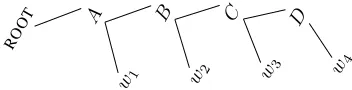
which is said to tag each word wj with its par-ent state. All parses share this right-branching tree structure, so they differ only in their choice of tags.
(Traditionally, the weight G(A → w B) or G(A→w)is defined as the product of anemission probability,p(w | A), and atransition probabil-ity, p(B | A) or p(HALT | A). However, the fol-lowing algorithms do not require this. Indeed, the algorithms do not require that G is a PCFG—any right-branching WCFG will do.)
In this setting, the inside algorithm (which com-putesβ bottom-up) is known as the backward al-gorithm, because it proceeds from right to left. The subsequent outside pass (which computes α top-down) is known as theforward algorithm.
Thanks to the fixed tree structure, this special-ized version of inside-outside can run in total time of onlyO(n|N |2). Of course, once we work out the
fast backward algorithm (directly or from the inside algorithm), the forward-backward algorithm comes for free by algorithmic differentiation, withα[x] de-notingðx=∂Z/∂x. Pseudocode appears as Algo-rithms 6–7 in Appendix B.
[image:9.612.333.509.185.230.2]via (1). Following section 7, one can determine tran-sition probabilities to the edges of the trellis so that a random walk on the trellis samples a tagging, from left to right, according to (1). The backward algo-rithm serves to computeβ values from which these transition probabilities are found (cf. section 7.1). Under these probabilities, the trellis becomes a non-stationary Markov model over the taggings. The for-ward pass now finds the hitting probabilities in this Markov model (cf. section 7.3), which describe how often the random walk will reach specific anchored nonterminals or traverse edges between them. These are the expected counts of tags and tag bigrams at specific positions.
8.2 Other grammar formalisms
Many grammar formalisms have weighted versions that produce exponential-family distributions over tree-structured derivations:
• PCFGs or WCFGs whose nonterminals are lex-icalized or extended with other attributes, in-cluding unification-based grammars (Johnson et al., 1999)
• Categorial grammars, which use an unbounded set of nonterminalsN (bounded for any given input sentence)
• Tree substitution grammars and tree adjoin-ing grammars (Schabes, 1992), in which the derivation tree is distinct from the derived tree • History-based stochasticizations such as the
structured language model (Jelinek, 2004) • Projective and non-projective dependency
grammars as mentioned earlier
• Semi-Markov models for chunking (Sarawagi and Cohen, 2004), with runtimeO(n2)
Each formalism has one or more inside algo-rithms10that efficiently computeZ, typically in time
O(n2) toO(n6) via dynamic programming. These
inside algorithms can all be differentiated using the same recipe.
The trick continues to work when one of these in-side algorithms is extended to the case of prefix pars-ing or lattice parspars-ing (Nederhof and Satta, 2003), where the input sentence is not fully observed, or
10Even basic WCFGs admit multiplealgorithms—Earley’s algorithm, unary cycle elimination, the “hook trick,” and more (see Goodman, 1998; Eisner and Blatz, 2007).
to partially supervised parsing (Pereira and Schabes, 1992; Matsuzaki et al., 2005), where the output tree is not fullyunobserved.
8.3 Synchronous grammars
In a synchronous grammar (Shieber and Schabes, 1990), a parseT is a derivation tree that produces aligned syntactic representations of a pair of sen-tences. These cases are handled as before. The in-put to the inside algorithm is a pair of aligned or unaligned sentences, or a single sentence.
The simplest synchronous grammar is a finite-state transducer. HereT is an alignment of the two sentences, tagged with states. Eisner (2002) general-ized the forward-backward algorithm to this setting and drew a connection to gradients.
8.4 Conditional grammars
In the conditional random field (CRF) approach, p(T | w) is defined as Gw(T)/Z, where Gw is a
specialized grammar constructed given the inputw. GenerallyGwdefines weights for theanchoredrules
R0, allowing the weight of a rule to be
position-specific. (This slightly affects lines 5 and 11 of Algorithm 1.) Any weighted grammar formalism may be used: e.g., the formalisms in section 2 and section 8.1 respectively yield the CRF-CFG (Finkel et al., 2008) and the popular linear-chain CRF (Sut-ton and McCallum, 2011).
Nothing in our approach changes. In fact, super-vised training of a CRF usually follows the gradi-ent∇logp(T∗ |w). This equals the vector of rule
counts observed in the supervised treeT∗, minus the
expected rule counts∇logZ—as equivalently com-puted by backproporinside-outside.
8.5 Pruned, prioritized, and beam parsing
For speed, it is common in practice to perform only a subset of the updates at line 11 of Algorithm 1. This approximate algorithm computes an underesti-mate Zˆ of Z (via underestimates βˆ[Ak
i]), because only a subset of the inside circuit is used. By storing this dynamically determined smaller circuit and performing back-propagation through it (Eisner et al., 2005), we can compute the partial deriva-tives∂Z/∂ˆ βˆ[Ak
in the pruned parse forest, which consists of the parse trees—with total weightZˆ—explored by the approximate algorithm.
Many clever single-pass or multi-pass strategies exist for including the most important updates. Strategies are usually based either on direct prun-ing of constituents or prioritized updates with early stopping. A key insight is thatβ[Ak
i]·ðβ[Aki]is the total contribution ofβ[Ak
i]to Z, so one should be sure to include the updateβ[Ak
i] += ∆if∆·α[Aki] is predicted to be large.
Weighted automata are popular for parsing, par-ticularly dependency parsing (Nivre, 2003). In this case,T is similar to a derivation tree: it is a sequence of operations (e.g., shift and reduce) that constructs a syntactic representation. Here an approximateZˆ is usually computed by beam search, and can be dif-ferentiated as above.
8.6 Inside-outside should be as fast as inside
In all cases, it is good practice to derive one’s inside-outside algorithm by differentiation—manual or automatic—to ensure correctness and efficiency.
It should be a red flag if a proposed inside-outside algorithm is asymptotically slower than its inside al-gorithm.11 Why? Because automatic differentiation
produces an adjoint circuit that is at most twice the size of the original circuit (assuming binary opera-tors). That means∇logZ alwayscanbe evaluated with the same asymptotic runtime aslogZ.
Good researchers do sometimes slip up and pub-lish less efficient algorithms. Koo et al. (2007) present theO(n3)algorithms for non-projective
de-pendency parsing: they point out that a contempo-raneous IWPT paper with the same O(n3) inside
algorithm had somehow raised inside-outside’s run-time fromO(n3) toO(n5). Similarly, Vieira et al.
(2016) provide efficient algorithms for variable-order linear-chain CRFs, but note that a JMLR pa-per with the same forward algorithm had raised the grammar constant in forward-backward’s runtime.
11Unless inside-outside has beendeliberatelyslowed down to reduce itsspacerequirements, as in the discard-and-recompute scheme of Zweig and Padmanabhan (2000). Absent such a scheme, inside-outside may need asymptotically more space than inside: though the adjoint circuit is not much bigger than the original, evaluating it may require keeping more of the orig-inal in memory at once (unless time is traded for space).
9 Conclusions and Further Reading
Computational linguists have been back-propagating through their arithmetic circuits for a long time without realizing it—indeed, since before Rumelhart et al. (1986) popularized the use of this technique to train neural networks. Recognizing this connection can help us to under-stand, teach, develop, and implement many core algorithms of the field.
Good follow-up reading includes
• how to use the inside algorithm within a larger neural network that can be differentiated end-to-end (Gormley et al., 2015; Gormley, 2015); • how to efficiently obtain the partial derivatives
of the expected counts by differentiating the al-gorithm a second time (Li and Eisner, 2009); • how to navigate through the space of possible
inside algorithms (Eisner and Blatz, 2007); • how to convert an inside algorithm into variant
algorithms such as Viterbi parsing,k-best pars-ing, and recognition (Goodman, 1999);
• how to apply the same ideas to graphical mod-els (Aji and McEliece, 2000; Darwiche, 2003).
Acknowledgments
A Pseudocode for Inside-Outside Variants
The core of this paper is Algorithms 1 and 2 in the main text. For easy reference, this appendix pro-vides concrete pseudocode for some close variants of Algorithm 2 that are discussed in the main text, highlighting the differences from Algorithm 2. All of these variants compute the same expected counts c, with only small constant-factor differences in ef-ficiency.
Algorithm 3 is the clean, efficient version of inside-outside that obtains the expected counts ∇logZ by direct implementation of backprop. We may regard this as the fundamental form of the algo-rithm. The differences from Algorithm 2 are high-lighted inredand discussed in section 6.1.
SincelogZis replacingZas the output being dif-ferentiated, the adjoint quantityðx is redefined as ∂(logZ)/∂x and stored in α
Z[x]. The name Zα is chosen because it is Z1 times the traditionalα. The computations in the loops are not affected by this rescaling: they perform the same operations as in Algorithm 2. Only the start and end of the algorithm are different (lines 4 and 17).
To emphasize the pattern of reverse-mode auto-matic differentiation, Algorithm 3 takes care to com-pute the adjoint quantities in exactly the reverse of the order in which Algorithm 1 computed the orig-inal quantities. The resulting iteration order in the i, j, and k loops is highlighted in blue. Comput-ing adjoints in reverse order always works and can be regarded as the default strategy. However, this is merely a cosmetic change: the version in Algo-rithm 2 is just as valid, because it too visits the nodes of the adjoint circuit in a topologically sorted order. Indeed, since each of these blue loops is paralleliz-able, it is clear that the order cannot matter. What is crucial is that the overall narrow-to-wide order of Algorithm 1, which isnotparallelizable, is reversed by both Algorithm 2 and Algorithm 3.
Algorithm 4 is a more traditional version of Al-gorithm 2. The differences from AlAl-gorithm 2 are highlighted inredand discussed in section 6.1.
Finally, Algorithm 5 is a version that is derived on independent principles (section 7.3). It directly
Algorithm 3A cleaner variant of the inside-outside algorithm
1: procedureINSIDE-OUTSIDE(G,w)
2: Z:=INSIDE(G,w) .side effect: setsβ[· · ·] 3: initialize allα[· · ·]to 0
4: Zα[ROOTn0] += Z1 .setsðZ = 1/Z
5: forwidth:=ndownto 2 : .wide to narrow
6: fori:=n−widthdownto0: .start point
7: k :=i+width .end point
8: forj:=k−1downtoi+ 1: .midpoint
9: forA, B, C ∈ N :
10: Zα[A→B C]+= Zα[Aik]β[Bij]β[Cjk] 11: Zα[Bij]+=G(A→B C)Zα[Aki]β[Cjk] 12: Zα[Cjk]+=G(A→B C)β[Bij]Zα[Aki] 13: fork:=ndownto1: .width-1 constituents
14: forA∈ N : p
15: Zα[A→wk] += αZ[Ak k−1]
16: forR∈ R: .expected rule counts
17: c(R) := αZ[R]· G(R) .no division byZ
Algorithm 4 A more traditional variant of the inside-outside algorithm
1: procedureINSIDE-OUTSIDE(G,w)
2: Z:=INSIDE(G,w) .side effect: setsβ[· · ·] 3: initialize allα[· · ·]to 0
4: α[ROOTn0] += 1 .setsðZ= 1 5: forwidth:=ndownto 2 : .wide to narrow
6: fori:= 0ton−width: .start point
7: k :=i+width .end point
8: forj:=i+ 1tok−1: .midpoint
9: forA, B, C ∈ N :
10: c(A→B C)
+= α[Aki]G(A→B C)β[Bij]β[Cjk]
Z 11: α[Bij]+=G(A→B C)α[Ak
i]β[Cjk]
12: α[Cjk]+=G(A→B C)β[Bij]α[Aki]
13: fork:= 1ton: .width-1 constituents
14: forA∈ N :
15: c(A→wk) += α[Akk−1]G(A→wk)
Z 16: forR∈ R:
computes the hitting probabilities of anchored con-stituents and rules in a PCFG representation of the parse forest. This may be regarded as the most natu-ral way to obtain the algorithm without using gradi-ents. However, as section 7.3 notes, it can be fairly easily rearranged into Algorithm 3, which is slightly more efficient. The differences from Algorithms 2 and 3 are highlighted inred.
To rearrange Algorithm 5 into Algorithm 3, the key is to compute not the countc(x), but the ratio c(x)
β[x] (or Gc((xx)) whenxis a rule), storing this ratio in
the variable α
Z[x]. This ratio Zα[x]can be interpreted as∂(logZ)/∂xas previously discussed.
Algorithm 5An inside-outside variant motivated as finding hitting probabilities
1: procedureINSIDE-OUTSIDE(G,w)
2: Z :=INSIDE(G,w) .side effect: setsβ[· · ·] 3: initialize allc[· · ·]to 0
4: c(ROOTn0) += 1
5: forwidth:=ndownto 2 : .wide to narrow
6: fori:= 0ton−width: .start point
7: k:=i+width .end point
8: forj:=i+ 1tok−1: .midpoint
9: forA, B, C ∈ N :
10: c(Aki→Bij Cjk) := .eqs.(19),(17)
c(Ak
i)·G(A→B C)·β[B
j i]·β[Cjk]
β[Ak i]
11: c(A→B C) += c(Aki →Bij Cjk) 12: c(Bij) += c(Aki →Bij Cjk) 13: c(Cjk) += c(Aki →Bij Cjk)
14: fork:= 1ton: .width-1 constituents
15: forA∈ N :
16: c(Akk−1→wk):=c(Akk−1) .eqs.(19),(18)
17: c(A →wk)+=c(Akk−1→wk)
18: forR∈ R: .expected rule counts
19: do nothing.c(R)has already been computed
B Pseudocode for Forward-Backward
Algorithm 6 is the backward algorithm, as intro-duced in section 8.1. It is an efficient specializa-tion of the inside algorithm (Algorithm 1) to right-branching trees.
Notation: We use ROOT0 to denote the root an-chored nonterminal, andAj (forA ∈ N and 1 ≤
j ≤ n) to denote an anchored nonterminal A that serves as the tag ofwj. That is, Aj is anchored so that its left child iswj. (Since thisAj actually dom-inates all ofwj. . . wnin the right-branching tree, it would be called An
j−1 if we were running the full
inside algorithm.)
Line 7 builds up the right-branching tree by com-bining a word from j −1 to j (namely wj) with a phrase fromj ton (namely Bj+1). This line is
a specialization of line 11 in Algorithm 1, which combines a phrase fromitoj with another phrase from j to k. Thanks to the right-branching con-straint, the backward algorithm only has to loop over O(n)triples of the form(j−1, j, n)(with fixedn)— whereas the inside algorithm must loop overO(n3)
triples of the form(i, j, k).
Algorithm 6The backward algorithm
1: functionBACKWARD(G,w) 2: initialize allβ[· · ·]to 0
3: forA∈ N : .stopping rules
4: β[An] += G(A→wn)
5: forj:=n−1downto1:
6: forA, B∈ N : .transition rules
7: β[Aj] += G(A→wj B)β[Bj+1]
8: forA∈ N : .starting rules
9: β[ROOT0] += G(ROOT→A)β[A1]
10: returnZ :=β[ROOT0]
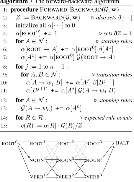
The forward-backward algorithm, Algorithm 7, is derived mechanically by differentiating Algo-rithm 6, by exactly the same procedure as in sec-tion 5. As a result, it is a specializasec-tion of Algo-rithm 2.
This presentation of the forward-backward algo-rithm finds the expected counts of rules R ∈ R. However, section 8.1 mentions that each ruleRcan be regarded as consisting of an emission actionRe
followed by a transition action Rt. We may want
to find the expected counts of the various actions. These can of course be found by summing the ex-pected counts of all rules containing a given action. However, this step can also be handled naturally by backprop, in the common case where eachG(R) is defined as a productpRe·pRtof the conditional
Algorithm 7The forward-backward algorithm
1: procedureFORWARD-BACKWARD(G,w)
2: Z :=BACKWARD(G,w) .also setsβ[· · ·] 3: initialize allα[· · ·]to 0
4: α[ROOT0] += 1 .setsðZ= 1
5: forA∈ N : .starting rules
6: α[ROOT→A] += α[ROOT0]β[A1]
7: α[A1] += α[ROOT0]G(ROOT→A)
8: forj:= 1ton−1:
9: forA, B∈ N : .transition rules
10: α[A→wj B] += α[Aj]β[Bj+1] 11: α[Bj+1] += α[Aj]G(A→wj B)
12: forA∈ N : .stopping rules
13: G(A→wn) += α[An]
14: forR∈ R: .expected rule counts
15: c(R) :=α[R]· G(R)/Z
ROOT0 ROOT1 ROOT2 ROOT3 HALT
NOUN1 NOUN2 NOUN3
[image:14.612.75.302.66.374.2]VERB1 VERB2 VERB3
Figure 1:The trellis of taggings of a length-3 sentence, under an HMM whereN = {ROOT,NOUN,VERB}. (Although the trellis shows thatROOTmay be used as an ordinary tag, often in practice it is allowed only at the root. This can be arranged by giving weight 0 to rules involvingROOTjforj >0, corre-sponding to the gray edges.)
as the sum of two parameters, θRe + θRt, which
represent the logs of these conditional probabilities. Then the expected emission and transition counts are given by∂(logZ)/∂θReand∂(logZ)/∂θRt.
It is traditional to view the forward-backward al-gorithm as running over a “trellis” of taggings (Fig-ure 1), which represents the forest of parses. Since a nonterminalAj that is anchored at positionj nec-essarily emitswj, the trellis representation does not bother to show the emissions. It is simply a directed graph showing the transitions. Every parse (tagging) ofwcorresponds to a path in Figure 1. Specifically, edgeAj → Bj+1 in the trellis represents the
an-chored ruleAj → wj Bj+1, without showing wj.
Similarly,An→ HALTrepresents the anchored rule An → wn, without showingwn, andROOT → A1
represents the anchored rule ROOT → A1. The weight of a trellis edge corresponding to an anchor-ing of rule Ris given by G(R). The weight G(T) of a taggingT is then the product weight of the path that corresponds to that tagging.
On this view, the inner weight β[Aj]can be re-garded as a suffix weight: it sums up the weight of all paths fromAj toHALT. Algorithm 6 can be transparently viewed as computing all suffix weights from right to left by dynamic programming. Z = ROOT0 sums the weight of all paths fromROOT0 to HALT. Similarly, the outer weightα[Aj]can be re-garded as aprefix weight, computed symmetrically within Algorithm 7.
The constructions of section 7 are easier to un-derstand in this setting. Here is the interpretation. It is possible to replace the non-negativeweightson the trellis edges with probabilities, in such a way that the product weight of each path is not changed. Indeed, the method is essentially identical to the “weight pushing” algorithm for weighted finite-state automata (Mohri, 2000).
The probabilistic version of the trellis is a repre-sentation of a new weighted grammarG0—an HMM
(hence a type of PCFG) that generates only taggings ofw, with the probabilities given by (1).
In the probabilistic version of the trellis, the edges from a node have total probability of 1. Thus it is the graph of a Markov chain, whose states are the anchored nonterminalsN0. Sampling a tagging of
w is now as simple as taking a random walk from ROOT0untilHALTis reached. The forward pass can be interpreted as a straightforward use of dynamic programming to compute the hitting probabilities of the nodes in the trellis, as well as the probabilities of traversing a node’s out-edges once the node is hit.
But how were the trellis probabilities found in the first place? The edge Aj → Bj+1 originally had
weightG(A → wj B). In the probabilistic version of the trellis, it has probability G(A→wjB)·β[Bj+1]
β[Aj] .
References
Steven Abney, David McAllester, and Fernando Pereira. Relating probabilistic grammars and automata. In
Pro-ceedings of ACL, pages 542–557, 1999.
S. Aji and R. McEliece. The generalized distributive law.
IEEE Transactions on Information Theory, 46(2):325–
343, 2000.
J. K. Baker. Trainable grammars for speech recognition. In Jared J. Wolf and Dennis H. Klatt, editors,Speech Communication Papers Presented at the 97th Meeting
of the Acoustical Society of America, MIT, Cambridge,
MA, June 1979.
Yehoshua Bar-Hillel, M. Perles, and E. Shamir. On for-mal properties of simple phrase structure grammars.
Zeitschrift f¨ur Phonetik, Sprachwissenschaft und
Kom-munikationsforschung, 14:143–172, 1961. Reprinted
in Y. Bar-Hillel. (1964).Language and Information:
Selected Essays on their Theory and Application,
Addison-Wesley 1964, 116–150.
L. E. Baum. An inequality and associated maximiza-tion technique in statistical estimamaximiza-tion of probabilistic functions of a Markov process.Inequalities, 3, 1972. Taylor Berg-Kirkpatrick, Alexandre Bouchard-Cˆot´e,
DeNero, John DeNero, and Dan Klein. Painless un-supervised learning with features. InProceedings of
NAACL, June 2010.
James Bergstra, Olivier Breuleux, Fr´ed´eric Bastien, Pas-cal Lamblin, Razvan Pascanu, Guillaume Desjardins, Joseph Turian, David Warde-Farley, and Yoshua Ben-gio. Theano: A CPU and GPU math compiler in python. In St´efan van der Walt and Jarrod Millman, editors,Proceedings of the 9th Python in Science
Con-ference, pages 3–10, 2010.
S. Billot and B. Lang. The structure of shared forests in ambiguous parsing. InProceedings of ACL, pages 143–151, April 1989.
Rens Bod. Enriching Linguistics with Statistics:
Per-formance Models of Natural Language. PhD thesis,
University of Amsterdam, Academische Pers, Amster-dam, 1995. ILLC Dissertation Series 1995-14. Zhiyi Chi. Statistical properties of probabilistic
context-free grammars. Computational Linguistics, 25(1): 131–160, 1999.
Adnan Darwiche. A differential approach to inference in Bayesian networks. Journal of the Association for
Computing Machinery, 50(3):280–305, 2003.
A. P. Dempster, N. M. Laird, and D. B. Rubin. Maximum likelihood from incomplete data via the EM algorithm.
J. Royal Statist. Soc. Ser. B, 39(1):1–38, 1977. With
discussion.
J. Earley. An efficient context-free parsing algorithm.
Communications of the ACM, 13(2):94–102, 1970.
Jason Eisner. Three new probabilistic models for de-pendency parsing: An exploration. InProceedings of
COLING, pages 340–345, Copenhagen, August 1996.
Jason Eisner. Parameter estimation for probabilistic finite-state transducers. InProceedings of ACL, pages 1–8, 2002.
Jason Eisner and John Blatz. Program transformations for optimization of parsing algorithms and other weighted logic programs. InProceedings of the 11th Conference
on Formal Grammar, pages 45–85, 2007.
Jason Eisner, Eric Goldlust, and Noah A. Smith. Compil-ing comp lCompil-ing: Weighted dynamic programmCompil-ing and the Dyna language. InProceedings of HLT-EMNLP, pages 281–290, 2005.
Jenny Rose Finkel, Christopher D. Manning, and An-drew Y. Ng. Solving the problem of cascading errors: Approximate Bayesian inference for linguistic annota-tion pipelines. InProceedings of EMNLP, pages 618– 626, 2006.
Jenny Rose Finkel, Alex Kleeman, and Christopher D. Manning. Efficient, feature-based, conditional random field parsing. InProceedings of ACL-08: HLT, pages 959–967, June 2008.
Christoph Goller and Andreas K¨uchler. Learning task-dependent distributed representations by backpropaga-tion through structure. Report AR-95-02, Fakult¨at F¨ur Informatik, Technischen Universit¨at M¨unchen, 2005. Joshua Goodman. Efficient algorithms for parsing the
DOP model. InProceedings of EMNLP, 1996. Joshua Goodman. Parsing Inside-Out. PhD thesis,
Har-vard University, May 1998.
Joshua Goodman. Semiring parsing.Computational
Lin-guistics, 25(4):573–605, December 1999.
Matthew R. Gormley. Graphical Models with Structured Factors, Neural Factors, and Approximation-Aware
Training. PhD thesis, Johns Hopkins University,
Oc-tober 2015.
Matthew R. Gormley, Mark Dredze, and Jason Eisner. Approximation-aware dependency parsing by belief propagation.Transactions of the Association for
Com-putational Linguistics, 3:489–501, August 2015. ISSN
2307-387X.
Andreas Griewank and George Corliss, editors.
Auto-matic Differentiation of Algorithms. SIAM,
Philadel-phia, 1991.
of Processing Techniques on Communication, pages 569–598. Martinus Nijhoff, 1985.
Frederick Jelinek. Stochastic analysis of structured lan-guage modeling. In Mark Johnson, Sanjeev P. Khu-danpur, Mari Ostendorf, and Roni Rosenfeld, editors,
Mathematical Founations of Speech and Languge
Pro-cesing, number 138 in IMA Volumes in Mathematics
and its Applications, pages 37–71. Springer, 2004. Mark Johnson, Stuart Geman, Stephen Canon, Zhiyi
Chi, and Stefan Riezler. Estimators for stochastic ‘unification-based’ grammars. InProceedings of ACL, pages 535–549, University of Maryland, 1999. Tadao Kasami. An efficient recognition and syntax
algo-rithm for context-free languages. Technical report, Air Force Cambridge Research Laboratory, 1965.
Dan Klein and Christopher D. Manning. Parsing and hy-pergraphs. InProceedings of the International
Work-shop on Parsing Technologies (IWPT), 2001.
Terry Koo, Amir Globerson, Xavier Carreras, and Michael Collins. Structured prediction models via the matrix-tree theorem. InProceedings of
EMNLP-CoNLL, pages 141–150, June 2007.
K. Lari and S. Young. The estimation of stochastic context-free grammars using the inside-outside algo-rithm. Computer Speech and Language, 4:35–56, 1990.
K. Lari and S. Young. Applications of stochastic context-free grammars using the inside-outside algorithm.
Computer Speech and Language, 5:237–257, 1991.
Yann LeCun. Une proc´edure d’apprentissage pour r´eseau a seuil asymmetrique (a learning scheme for asymmet-ric threshold networks). InProceedings of Cognitiva 85, pages 599–604, Paris, France, 1985.
Zhifei Li and Jason Eisner. First- and second-order ex-pectation semirings with applications to minimum-risk training on translation forests. InProceedings of
EMNLP, pages 40–51, 2009.
Takuya Matsuzaki, Yusuke Miyao, and Jun’ichi Tsujii. Probabilistic CFG with latent annotations. In
Proceed-ings of ACL, pages 75–82, 2005.
David McAllester, Michael Collins, and Fernando Pereira. Case-factor diagrams for structured proba-bilistic modeling. InProceedings of UAI, 2004. Mehryar Mohri. Minimization algorithms for sequential
transducers. Theoretical Computer Science, 324:177– 201, March 2000.
Mark-Jan Nederhof and Giorgio Satta. Probabilistic pars-ing as intersection. InProceedings of the 8th
Inter-national Workshop on Parsing Technologies (IWPT),
pages 137–148, April 2003.
Joakim Nivre. An efficient algorithm for projective de-pendency parsing. In Proceedings of the 8th
Inter-national Workshop on Parsing Technologies (IWPT),
pages 149–160, 2003.
Fernando Pereira and Yves Schabes. Inside-outside rees-timation from partially bracketed corpora. In Proceed-ings of ACL, 1992.
D. E. Rumelhart, G. E. Hinton, and R. J. Williams. Learn-ing internal representations by error propagation. In D. E. Rumelhart and J. L. McClelland, editors, Par-allel Distributed Processing: Explorations in the
Mi-crostructure of Cognition, volume 1, pages 318–362.
MIT Press, 1986.
Ruslan Salakhutdinov, Sam Roweis, and Zoubin Ghahra-mani. Optimization with EM and expectation-conjugate-gradient. InProceedings of ICML, Wash-ington, DC, 2003.
Sunita Sarawagi and William W Cohen. Semi-Markov conditional random fields for information extraction.
InProceedings of NIPS, 2004.
Taisuke Sato. A statistical learning method for logic pro-grams with distribution semantics. InProceedings of ICLP, pages 715–729, 1995.
Taisuke Sato and Yoshitaka Kameya. New advances in logic-based probabilistic modeling by PRISM. In
Probabilistic Inductive Logic Programming, pages
118–155. Sringer, 2008.
Yves Schabes. Stochastic lexicalized tree-adjoining grammars. InProceedings of COLING, 1992. Stuart Shieber and Yves Schabes. Synchronous
tree-adjoining grammars. In Proceedings of COLING, 1990.
David A. Smith and Noah A. Smith. Probabilistic models of nonprojective dependency trees. InProceedings of
EMNLP-CoNLL, pages 132–140, 2007.
Andreas Stolcke. An efficient probabilistic context-free parsing algorithm that computes prefix probabilities.
Computational Linguistics, 21(2):165–201, 1995.
Charles Sutton and Andrew McCallum. An introduction to conditional random fields. Foundations and Trends
in Machine Learning, 4(4):267–373, 2011.
Richard A. Thompson. Determination of probabilis-tic grammars for functionally specified probability-measure languages.IEEE Transactions on Computers, C-23(6):603–614, 1974.
Tim Vieira, Ryan Cotterell, and Jason Eisner. Speed-accuracy tradeoffs in tagging with variable-order CRFs and structured sparsity. In Proceedings of
K. Vijay-Shankar, David J. Weir, and Aravind K. Joshi. Characterizing structural descriptions produced by various grammatical formalisms. In Proceedings of ACL, pages 104–111, 1987.
K. Vijay-Shanker and David J. Weir. Parsing some con-strained grammar formalisms.Computational Linguis-tics, 19(4):591–636, 1993.
Michael D. Vose. A linear algorithm for generating random numbers with a given distribution. IEEE
Transactions on Software Engineering, 17(9):972–
975, September 1991.
P. Werbos.Beyond Regression: New Tools for Prediction
and Analysis in the Behavioral Sciences. PhD thesis,
Harvard University, 1974.
Ronald J. Williams and David Zipser. A learning al-gorithm for continually running fully recurrent neural networks.Neural Computation, 1(2):270–280, 1989. D. H. Younger. Recognition and parsing of context-free
languages in timen3.Information and Control, 10(2):
189–208, February 1967.